 2021, Vol. 39
Institute of Oceanology, Chinese Academy of Sciences
Article Information
- WANG Tongyu, ZHANG Shuwen, CHEN Fajin, MA Yonggui, JIANG Chen, YU Jie
- Influence of sequential tropical cyclones on phytoplankton blooms in the northwestern South China Sea
- Journal of Oceanology and Limnology, 39(1): 14-25
- http://dx.doi.org/10.1007/s00343-020-9266-7
Article History
- Received Oct. 17, 2019
- accepted in principle Dec. 10, 2019
- accepted for publication Feb. 4, 2020


2 Institute of Marine Science, Shantou University, Shantou 515063, China;
3 Laboratory for Regional Oceanography and Numerical Modeling, Qingdao National Laboratory for Marine Science and Technology, Qingdao 266000, China
The western North Pacific see the largest number of tropical cyclones annually, and their intensity is also greater with respect to other cyclone-rich basins. Typhoons that pass through the South China Sea (SCS) landed in Guangdong Province and Hainan Province of China, and Vietnam. Strong winds and heavy rains posed a huge threat in the coastal areas (Chen et al., 2013). They occurred about 10 times a year over SCS, mostly between July and October. However, the sequential tropical cyclones are relatively rare over the SCS.
When a tropical cyclone transits the sea surface, sea surface cooling (SSC) is one of the most apparent features of air-sea interactions, and has an important impact on the upper ocean temperature distribution and the exchange of air-sea heat flux. In particular, the SSC may last for more than two weeks and affect atmospheric circulation on a large scale (Hart et al., 2007; Liu et al., 2008). Simultaneously, the SSC also has a significant negative feedback effect on the tropical cyclone intensity, weakening or possibly even closing the energy supply to tropical cyclone (Timmermann et al., 2005; Soloviev et al., 2014). According to the observed records, the tropical cyclone can generally reduce the sea surface temperature (SST) by 2–6 ℃ (D'Asaro, 2003; Lin et al., 2013; Zhang et al., 2014). Typhoon Kai-Tak in 2000 was an exception, the maximum SSC over SCS was 10.8 ℃ (Chiang et al., 2011). There is still considerable controversy about the driving mechanism that permits a tropical cyclone to give rise to SSC. Some studies have suggested that the SSC is mainly driven by tropical cyclone induced Ekman pumping (Babin et al., 2004; Chiang et al., 2011; Zhao et al., 2013; Guan et al., 2014). Some scientists believe that the combined effect of turbulent mixing and upwelling is the primary cooling mechanism (Price et al., 1994; Dickey et al., 1998; D'Asaro et al., 2007; Price, 2009; Zhang et al., 2016), with air-sea fluxes playing a minor role (Price, 1981). Other researchers hold the viewpoint that SSC is mainly a result of the turbulent mixing caused by tropical cyclones (Price, 1981; Jacob et al., 2000; Sriver and Huber, 2007; Zhang et al., 2014). At present, owing to the lack of effective in situ measurements obtained under tropical cyclone forcing conditions, there is still no convincing observational evidence that can be used to determine whether upwelling or turbulent mixing is the main driving mechanism for the SSC. More importantly, tropical cyclones also exert a major influence on the marine ecosystem (Subrahmanyam et al., 2002; Lin et al., 2003, 2008; Shi and Wang, 2007; Zheng and Tang, 2007; Shang et al., 2008; Zhao et al., 2008; Sun et al., 2010; Zhao et al., 2017; Wu and Li, 2018). Recent work by Zhang et al. (2014) indicated that the nearinertial turbulence mixing induced by tropical storm can promote the exchange of nutrients fluxes between the deep layer and the upper ocean. The passage of a tropical cyclone usually induces near-inertial turbulent mixing and upwelling. All these physical processes can bring deep nutrient-rich cold waters to the upper ocean, where nutrients are scarce. The roles that tropical cyclone induced near-inertial turbulent mixing or upwelling plays in phytoplankton blooms remains unclear.
While oceanic responses to the passage of individual tropical cyclones have been extensively studied, very few studies have focused on sequential tropical cyclones (Wu and Li, 2018). In 2011, the rare phenomenon of three sequential tropical cyclones Haitang (September 24), Nesat (September 29) and Nalgae (October 3), provided a unique opportunity to study the upper ocean responses to the three sequential tropical cyclones in SCS. The objective of this study is to reveal the upper ocean responses to sequential tropical cyclones and associated physical mechanisms for the SSC and phytoplankton blooms in the northwest region of SCS. The manuscript is organized as follows: the data and methods are introduced in Section 2, results are presented in Section 3, discussions are reserved for Section 4, and conclusions are in Section 5.
2 DATA AND METHOD 2.1 Tropical storm Haitang, typhoons Nesat and NalgaeAccording to the best typhoon track data provided by the Shanghai Typhoon Research Institute, nine typhoons entered the SCS in 2011, two of which were generated locally, and the rest originated in the western Pacific Ocean. Typhoons 17 (Nesat) and 19 (Nalgae), and tropical storm 18 (Haitang) were generated successively from September to October 2011. Typhoon Nesat generated at 00:00 on September 23 (13°N, 139°E), with a central pressure and maximum wind speed of 1 004 hPa and 12 m/s, respectively (Fig. 1). At 00:00 on September 25, it became a strong tropical storm of central pressure and maximum wind speed of 985 hPa and 28 m/s, respectively, before strengthening into a typhoon at 18:00 on September 25, with its central pressure of 975 hPa and maximum wind speed of 33 m/s. It continued to strengthen to reach a strong typhoon level with its central pressure and maximum wind speed of 950 hPa and 45 m/s, respectively. Typhoon Nesat entered the SCS and began to weaken after landing in the Philippines, and landing on Hainan Island 3 days later with a maximum wind speed of 25 m/s. Tropical Storm Haitang generated at 18:00 on September 23 (16.2°N, 110°E), with a central pressure of 998 hPa and a maximum wind speed of 15 m/s. The wind speed reached a maximum of 18 m/s at 00:00 on September 25 in the area of the Xisha Islands, and then landed on Vietnam. Typhoon Nalgae generated at 12:00 on September 26 at 18°N, 139°E and moved northwestward, following a trajectory that was similar to that of typhoon Nesat. The central pressure reached 950 hPa when landing Luzon Island at 18:00 on September 30, with a maximum wind speed of 38 m/s. Wind speed began to decrease as typhoon Nalgae entered the SCS, and became a strong tropical storm level at 18:00 on October 1. It landed on Hainan Island at 18:00 on October 3. Nalgae landed on Hainan Island 4 days after Nesat.

|
| Fig.1 The tracks of three sequential typhoons in the SCS in 2011 Time interval between adjacent circles is 6 h. Colors of the circle indicates typhoon intensity. Star indicates location of the mooring site. |
The 10-m wind speed data were obtained from the Cross-Calibrated Multi-Platform data (Wentz et al., 2015) with a spatial and temporal resolution of 0.25°×0.25° and 6 h, respectively. The wind speed was produced from a combination of satellite data, moored buoy data and modeled wind data, the wind speeds was used to calculate the wind field of tropical cyclones as well as Ekman pumping velocity. The MW-IR Optimally Interpolated (OI) SST daily product was provided by Remote Sensing Systems, which combined the through-cloud capability of the microwave data (MW) with the high spatial resolution of the IR SST data, and had better spatial coverage of daily data. It had a daily temporal resolution including ascending and descending orbit segments. The daily average value was obtained by averaging the ascending and descending passes or assigning the available one if only one pass was available. The SST data was from December 1997 to 2017. These datasets were able to resolve unstable waves in the tropics and the cold wake of the sea when typhoon passed (Wentz et al., 2000).
Merged chlorophyll-a (chl-a) concentration data from three ocean color sensors (MODIS-Aqua, MERIS and SeaWiFS) were retrieved using the Garver-Siegel-Maritorena (GMS) algorithm (Maritorena et al., 2010). The daily chl-a data used in this study have a spatial resolution of 9 km.
We used Argo reanalysis data to calculate buoyancy frequency. The data were selected from the Global Ocean Argo gridded dataset (BOA_Argo) (Li et al., 2017) with a horizontal resolution of 1°×1° and 58 vertical standard layers down to 1975 dbar.
2.3 Mooring observations dataA mooring array had been deployed at 16°51.374′N, 112°19.118′E, near the Xisha Islands in the northwestern SCS for 143 days from August 1 to December 21 2011. The depth of the mooring site was 1 491 m. At the depth of 460 m, the mooring array station was equipped with a 75-kHz upward-looking acoustic Doppler current profiler (ADCP) for measuring the velocity profiles. Vertical sampling interval was 16 m, and the measurement frequency was 1 800 Hz, and effective measurement of water depth was 58–442 m. During the period of deployment, three sequential tropical cyclones, tropical storm Haitang, typhoons Nesat, and Nalgae, passed near the mooring station. The time interval between the three typhoons passing through the mooring station was 5 days and 4 days, respectively.
2.4 Calculation method of upwelling and eddy diffusivityEkman transport is governed by the balance of the wind stress and Coriolis force in the horizontal plane, resulting in the convergence and divergence of sea water at the Ekman pumping velocity (EPV), EPV can be calculated as (Price, 1981)
 (1)
(1)where f=2ωsinθ is the Coriolis parameter, ω is the rotational velocity of the Earth, θ is the latitude, ρ is the density of the ocean, and 
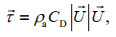 (2)
(2)where ρa is the density of air, 
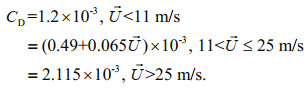 (3)
(3)Parameterization of the rate of dissipation of turbulent kinetic energy in the continental shelf ocean region is expressed as (Mackinnon and Gregg, 2003)
 (4)
(4)where N0=S0=3 cph, ε0=10-8 W/kg, Slf is the lowfrequency shear of background velocity, and N is the buoyancy frequency, which can be calculated from the BOA_Argo temperature and salt content products (Lu et al., 2018). Eddy diffusivity κρ can be derived from (Osborn, 1980)
 (5)
(5)where Γ is the mixing coefficient, we take it as 0.2 in this study.
3 RESULT 3.1 Response of SSTFigure 2 shows SST evolutions during the passage of tropical storm Haitang, typhoons Naset and Nalgae from September 21 to November 2, 2011 in the northwestern region of SCS. Before tropical storm Haitang arrived, the SST of the northwestern region of SCS was generally higher than 29 ℃ (Fig. 2a). When tropical storm Haitang passed through the mooring area, the SST dropped by more than 2 ℃ (Fig. 2b & c). Figure 2d shows the response of SST to typhoon Nesat. Compared with Fig. 2c, the cooling area enlarged significantly, the second day was the largest SST drop (SSC>5 ℃) on the right side of the typhoon track. Over the following days, the low temperature area decreased dramatically (Fig. 2e). When the typhoon Nalgae passed through the mooring area, however, the area of low temperature strengthened again, and the mean SST dropped by 2.2 ℃ (Fig. 2f). Over the next 10 days, the sea surface heated up again, SST increased by 1.2 ℃, and the area of low temperature was greatly reduced once more (Fig. 2g). But two weeks later, the area of low temperature expanded again, the greatest SST dropped was more than 2 ℃ (Fig. 2h). It should be noted that, after the passage of the three sequential tropical cyclones, the low temperature region lasted for more than 38 days in the northwestern of SCS where the mooring observation system located (Fig. 3). Whether this is in response to upwelling or other physical mechanisms will be discussed in the next section.

|
| Fig.2 Horizontal distribution of SST in the SCS in 2011 on the following dates a. September 21; b. September 26; c. September 27; d. September 29; e. October 1; f. October 4; g. October 15; h. November 2. Black lines represent typhoon tracks. Time interval between adjacent dots is 6 h. |

|
| Fig.3 Differences in SST in 2011 between September 21 and the following dates a. September 26 (after tropical storm Haitang); b. September 29 (after typhoon Nesat); c. October 4 (after typhoon Nalgae); d. November 2 (after strong upper ocean mixing). Black lines represent typhoon tracks. Time interval between adjacent dots is 6 h. |
The time series of observation was more than 45 days during the transition from late summer (September) to mid-autumn (November). The seasonal variation may be important for such a long period. In order to clarify the role of seasonal variations in the process of SSC, we calculated climatological SST from September 21 to November 2 during 1998–2017 (Fig. 4). The climatological SST decreased by about 1 ℃ from September 23 to November 10 due to seasonal change. At the same time, however, the SST in 2011 was less than 1.5 ℃ above the climatological SST.

|
| Fig.4 Temporal variation of the SST, in the area of the mooring site in 2011 A time series of climatological values is added as a reference. |
From the end of September to early of October, three tropical cyclones passed through the mooring area at intervals of 5 d and 4 d, respectively. After sequential tropical storm, as shown in Fig. 5, there were two phytoplankton blooms, with the first appeared on the 7th days after the passage of Nalgae, as evident by the surface chl-a concentration increased by 226%; and the second large-scale phytoplankton bloom emerged on 30th days after typhoon Nalgae, as evident by the surface chl-a concentration increased by 290% (Fig. 6). The possible driving mechanisms for the phytoplankton blooms will be analyzed in the next section.

|
| Fig.5 The average distribution of sea surface chl-a concentration in SCS in 2011 a. September 15-24; b. October 3-22; c. October 26–November 5. |
We also calculated climatological surface chl-a concentration from September 21 to November 2 during 1998–2017 year as a reference (Fig. 6). The climatological surface chl-a concentration changed little during this period.

|
| Fig.6 Temporal variation of the sea surface chl a in the area of the mooring site in 2011 A time series of climatological values is added as a reference. |
Previous studies have suggested that the SSC and phytoplankton blooms after the passage of typhoon are closely related to Ekman pumping induced by typhoon (Babin et al., 2004; Zhao et al., 2008; Chiang et al., 2011). Here, Eqs.1–2 were used to calculate the value of EPV caused by typhoon. As shown in Fig. 7, the intensity of Ekman pumping on both sides of the typhoon path was quite different. The upwelling in the right-hand side was not only stronger than left-hand side, but also larger in extent. As suggested by Price (1981) that the rightward bias of the SST drop due to the resonance of rotation of the wind vector with wind-driven inertial currents. In the three tropical cyclones, typhoon Nesat induced the strongest value of EPV, the maximum value of EPV was 1.8×10⁻⁴ m/s on September 29 (Fig. 7c). This was closely related to the sustained low temperature region before the midOctober (Fig. 2f) and the first phytoplankton bloom in early October (Fig. 6). After the passage of typhoon Nalgae, on November 2, EPV dropped to 5×10⁻⁶ m/s in the mooring area (Fig. 7f), which is about two orders of magnitude smaller than that measured during typhoon Nesat. Therefore, we can deduce that there must be other physical mechanisms that play a key role in processes of the SSC and the second phytoplankton bloom after mid-October.

|
| Fig.7 Variations of Ekman pumping velocity in the northwestern region of SCS from September–October 2011 a. 12.00 on September 24; b. 00.00 on September 28; c. 00.00 on September 29; d. 18.00 on October 2; e. 06.00 on October 3; f. 00.00 on November 2. All times are for UTC. The colors and arrows indicate the magnitude of the EPV and 10-m wind direction, respectively. Time interval between adjacent dots is 6 h, red dot represents typhoon position. |
The ADCP observational dataset were used to calculate the eastward and northward baroclinic velocities and their vertical profile of power spectrum. As shown in Fig. 8, The eastward baroclinic velocity power spectrum was very similar to that of northward baroclinic velocity. Moreover, the baroclinic energy dominated the whole water depth at a frequency of 10-5 Hz, this was roughly equal to the local inertial frequency. This implied that the existence of nearinertial oscillations (NIO) induced by tropical cyclones. To further analyze the NIO signal, nearinertial velocities within (0.8–1.2 f) were extracted by using a second-order Butterworth filter applied in the time domain (Kunze, 1985). The tropical storm Haitang and typhoons Nesat and Nalgae all induced NIOs (Fig. 9a). Haitang induced weak NIO signal and near-inertial energy that was distributed only in the upper 100 m (Fig. 9a). Both typhoons Nesat and Nalgae induced strong near-inertial flows. The nearinertial flow contour (isophase line) between October 4 and 19 exhibited a consistent slope (indicated by the green ellipse in Fig. 9a), and was used to estimate vertical phase velocity of the near-inertial wave. The average vertical phase velocities of the near-inertial internal waves induced by typhoons Nesat and Nalgae were 0.25 m/s and 0.12 m/s, respectively. Propagation time of near-inertial energy was 25 days for Nesat and 28 days for Nalgae. On the basis of propagation depth and time, we infer that NIOs that occurred on October 4 were generated by typhoon Nesat and those that occurred on October 21 were generated by typhoon Nalgae. Typhoon Nesat induced a maximum nearinertial velocity of 0.3 m/s at a depth of 186 m, while typhoon Nalgae induced a near-inertial velocity of 0.26 m/s at a depth of 122 m (Fig. 9a).

|
| Fig.8 Power spectrum of eastward (a) and northward (b) baroclinic velocities in the depth range of 58–442 m at the mooring site in 2011 |

|
| Fig.9 Profiles of the eastward near-inertial velocity (a), the northward velocity shear (b), and near-inertial energy distribution at mooring site (c) The two dotted lines denote the times when the typoons Nesat or Nalgae arrived. The green and yellow elliptical regions are the vertical shear induced by typhoons Nesat and Nalgae. |
The near-inertial wave induced by typhoon Nesat had a vertical wavelength of about 350 m, which was twice that induced by typhoon Nalgae. The horizontal scale of the near-inertial internal wave induced by typhoon Nesat reached 50 km, but that induced by typhoon Nalgae was less than 20 km. Wind forcing injects energy into the ocean and is distributed to different modes of ocean motions, and part of this energy input is dissipated at the bottom of mixed layer and in the thermocline, and the rest penetrates the thermocline into the deeper layer waters (D'Asaro et al., 1995). Downward transport of energy induced by typhoons Nesat and Nalgae reached strongest at water depth of 180 m and 130 m, respectively. It should be emphasized that, as shown in Fig. 9, the strongest velocity shear triggered by typhoon Nalgae was about 2 times larger than that of Nesat, while the nearinertial energy transmitted by typhoon Nesat was deeper than that of typhoon Nalgae. This suggests that typhoon Nalgae had dissipated more near-inertial energy in the upper ocean through the shear instability mechanism rather than typhoon Nesat. In order to clarify which is more important, winter monsoon or near-inertial mixing, we calculated the wind stress in the area of the mooring station for September 23 to December 31 in 2011. As shown in the Fig. 10, the winter monsoon was prevailing between late November and December. Prior to November 12, the value of wind stress was relatively steady and weak, and therefore unlikely to induce strong turbulent mixing. Apart from the decrease in SST, phytoplankton bloom associated with primary production was another obvious response to the passage of the tropical cyclones. On the one hand, near-inertial mixing raised the high chl-a concentrations in the subsurface to the surface layer, on the other hand, strong turbulent mixing can break up the barrier of the thermocline, and enhanced the exchange fluxes of nutrients from the deeper layer into the euphotic layer. During the passages of typhoons Nesat and Nalgae, the diapycnal flux of nutrients could be calculated by
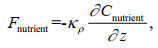

|
| Fig.10 Temporal variation of the wind stress in the area of the mooring site in 2011 |
where Cnutrient is the nutrient concentration. For constant 

|
| Fig.11 Profiles of the eddy diffusivity κρ in the area of the mooring site in 2011 The three dotted lines denote the times when the tropical storm Haitang, and typhoons Nesat and Nalgae arrived, respectively. |
An obvious question is why the chl-a concentrations declined from October 8 to 19. This may be due to two reasons:
(1) The EPV induced by typhoons rapid declined from 1.8×10⁻⁴ m/s on September 29 to 5×10⁻⁶ m/s on November 2. This implied that the nutrients transport by Ekman pumping was inadequate after the passage of typhoon Nalgae.
(2) As shown in Fig. 11, the eddy diffusivity induced by near-inertial oscillations was weak in the upper ocean between October 8 and 12. As a result, the vertical nutrient transport capacity by both upwelling and near-inertial mixing was weak, possibly resulting in the observed decrease in chl a. However, after October 13, chl a began to increase as near-inertial mixing began to intensify.
5 CONCLUSIONIn this study, the effects of tropical storm Haitang, typhoons Nesat, and Nalgae in 2011, on the distributions of SST and chl-a concentrations were investigated in the northwestern SCS using satellite remote sensing data, Argo reanalysis data, and a mooring array dataset. We found that, after the three sequential tropical cyclones, the low temperature region in the northwestern SCS lasted for 38 days, and more importantly, there were two phytoplankton blooms appeared in the same region. The first phytoplankton bloom occurred on the 7th day after typhoons. The second phytoplankton bloom occurred on the 30th day, which is the key discovery in this study. We proposed that the upwelling induced by typhoons were responsible for the SSC before midOctober and the first phytoplankton bloom in October 8. A dynamic analysis demonstrated that the low temperature region of northwestern of SCS still continued to maintain after mid-October and the second phytoplankton bloom in November 4 were the result of the strong near-inertial turbulent mixing induced by typhoons Nesat and Nalgae. The mean eddy diffusivity after the passage of typhoon Nesat was above 10-4 m2/s, which is one order of magnitude greater than the mean eddy diffusivity of the open ocean. The enhancement of the turbulent mixing in the upper ocean was conducive to transportation of nutrient-rich cold waters from the deep layer to the euphotic layer, leading to the long-term maintenance of the low temperature region as well as the second phytoplankton bloom in the northwestern region of the SCS.
6 DATA AVAILABILITY STATEMENTAll data generated and/or analyzed during this study are available on request from the corresponding author and first author.
7 ACKNOWLEDGMENTThe authors are grateful for the anonymous reviewers' careful review and constructive suggestions to improve the manuscript. We acknowledge the GlobColour Project for the chl-a data (http://globcolour.info), Remote Sensing Systems (http://www.remss.com/) for SST and 10-m wind data, the Global Ocean Argo gridded dataset (BOA_Argo) (http://www.argo.org.cn/english) for Argo reanalysis data, the Shanghai Typhoon Research Institute (http://typhoon.nmc.cn/) for information of typhoons.
Babin S M, Carton J A, Dickey T D, Wiggert J D. 2004. Satellite evidence of hurricane-induced phytoplankton blooms in an oceanic desert. J. Geophys. Res. Oceans, 109(C3): C03043.
DOI:10.1029/2003JC001938 |
Chen D K, Lei X T, Wang W, Wang G H, Han G J, Zhou L. 2013. Upper ocean response and feedback mechanisms to typhoon. Adv. Earth Sci., 28(10): 1 077-1 086.
DOI:10.11867/j.issn.1001-8166.2013.10.1077 |
Chiang T L, Wu C R, Oey L Y. 2011. Typhoon Kai-Tak:an ocean's perfect storm. J. Phys. Oceanogr., 41(1): 221-233.
DOI:10.1175/2010JPO4518.1 |
D'Asaro E A, Eriksen C C, Levine M D, Paulson C A, Niiler P, Van Meurs P. 1995. Upper-ocean inertial currents forced by a strong storm. Part I:data and comparisons with linear theory. J. Phys. Oceanogr., 25(11): 2 909-2 936.
DOI:10.1175/1520-0485(1995)025<2909:UOICFB>2.0.CO;2 |
D'Asaro E A, Sanford T B, Niiler P P, Terrill E J. 2007. Cold wake of hurricane Frances. Geophys. Res. Lett., 34(15): L15609.
DOI:10.1029/2007GL030160 |
D'Asaro E A. 2003. The ocean boundary layer below Hurricane Dennis. J. Phys. Oceanogr., 33(3): 561-579.
DOI:10.1175/1520-0485(2003)033<0561:TOBLBH>2.0.CO;2 |
Dickey T, Frye D, McNeil J, Manov D, Nelson N, Sigurdson D, Jannasch H, Siegel D, Michaels T, Johnson R. 1998. Upper-ocean temperature response to Hurricane Felix as measured by the Bermuda testbed mooring. Mon. Wea.Rev., 126(5): 1 195-1 201.
DOI:10.1175/1520-0493(1998)126<1195:UOTRTH>2.0.CO;2 |
Guan S D, Zhao W, Huthnance J, Tian J W, Wang J H. 2014. Observed upper ocean response to typhoon Megi (2010)in the Northern South China Sea. J. Geophys. Res.Oceans, 119(5): 3 134-3 157.
DOI:10.1002/2013JC009661 |
Hart R E, Maue R N, Watson M C. 2007. Estimating local memory of tropical cyclones through MPI anomaly evolution. Mon. Wea. Rev, 135(12): 3 99-4 005.
DOI:10.1175/2007MWR2038.1 |
Jacob S D, Shay L K, Mariano A J, Black P G. 2000. The 3D oceanic mixed layer response to Hurricane Gilbert. J.Phys. Oceanogr., 30(6): 1 407-1 429.
DOI:10.1175/1520-0485(2000)030<1407:TOMLRT>2.0.CO;2 |
Kunze E. 1985. Near-inertial wave propagation in geostrophic shear. J. Phys. Oceanogr., 15(5): 544-565.
DOI:10.1175/1520-0485(1985)015<0544:NIWPIG>2.0.CO;2 |
Li H, Xu F, Zhou W, Wang D, Wright J S, Liu Z, Lin Y. 2017. Development of a global gridded Argo data set with Barnes successive corrections. J. Geophys. Res. Oceans, 122.
DOI:10.1002/2016JC012285.6 |
Lin I I, Black P, Price J F, Yang C Y, Chen S S, Lien C C, Harr P, Chi N H, Wu C C, D'Asaro E A. 2013. An ocean coupling potential intensity index for tropical cyclones. Geophys. Res. Lett., 40(9): 1 878-1 882.
DOI:10.1002/grl.50091 |
Lin I I, Wu C C, Pun I F, Ko D S. 2008b. Upper-ocean thermal structure and the western North Pacific category 5 typhoons.Part I:ocean features and the category 5 typhoons' intensification.. Mon. Wea. Rev., 136(9): 3 288-3 306.
DOI:10.1175/2008MWR2277.1 |
Lin I, Liu W T, Wu C C, Wong G T, Hu C M, Chen Z Q, Liang W D, Yang Y, Liu K K. 2003. New evidence for enhanced ocean primary production triggered by tropical cyclone. Geophys. Res. Lett., 30(13): 1 718.
DOI:10.1029/2003GL017141 |
Liu L L, Wang W, Huang R X. 2008. The mechanical energy input to the ocean induced by tropical cyclones. J. Phys.Oceanogr., 38(6): 1 253-1 266.
DOI:10.1175/2007JPO3786.1 |
MacKinnon J A, Gregg M C. 2003. Mixing on the late-summer New England shelf-Solibores, shear, and stratification. J.Phys. Oceanogr., 33(7): 1 476-1 492.
DOI:10.1175/1520-0485(2003)033<1476:MOTLNE>2.0.CO;2 |
Maritorena S, d'Andon O H F, Mangin A, Siegel D A. 2010. Merged satellite ocean color data products using a biooptical model:characteristics, benefits and issues. Remote Sens. Environ., 114(8): 1 791-1804.
DOI:10.1016/j.rse.2010.04.002 |
Osborn T R. 1980. Estimates of the local rate of vertical diffusion from dissipation measurements. J. Phys.Oceanogr., 10(1): 83-89.
DOI:10.1175/1520-0485(1980)010<0083:EOTLRO>2.0.CO;2 |
Powell M D, Vickery P J, Reinhold T A. 2003. Reduced drag coefficient for high wind speeds in tropical cyclones. Nature, 422(6929): 279-283.
DOI:10.1038/nature01481 |
Price J F, Sanford T B, Forristall G Z. 1994. Forced stage response to a moving hurricane. J. Phys. Oceanogr., 24(2): 233-260.
DOI:10.1175/1520-0485(1994)024<0233:FSRTAM>2.0.CO;2 |
Price J F. 1981. Upper ocean response to a hurricane. J. Phys.Oceanogr., 11(2): 153-175.
DOI:10.1175/1520-0485(1981)011<0153:UORTAH>2.0.CO;2 |
Price J F. 2009. Metrics of hurricane-ocean interaction:vertically-integrated or vertically-averaged ocean temperature?. Ocean Sci, 5(3): 351-368.
DOI:10.5194/os-5-351-2009 |
Shang S L, Li L, Sun F Q, Wu J Y, Hu C M, Chen D W, Ning X R, Xing Y, Zhang C Y, Shang S P. 2008. Changes of temperature and bio-optical properties in the South China Sea in response to Typhoon Lingling, 2001. Geophys. Res. Lett., 35(10): L10602.
DOI:10.1029/2008GL033502 |
Shi W, Wang M H. 2007. Observations of a Hurricane Katrina-induced phytoplankton bloom in the Gulf of Mexico. Geophys. Res. Lett., 34(11): L11607.
DOI:10.1029/2007GL029724 |
Soloviev A V, Lukas R, Donelan M A, Haus B K, Ginis I. 2014. The air-sea interface and surface stress under tropical cyclones. Sci. Rep., 4(1): 5 306.
DOI:10.1038/srep05306 |
Sriver R L, Huber M. 2007. Observational evidence for an ocean heat pump induced by tropical cyclones. Nature, 447(7144): 577-580.
DOI:10.1038/nature05785 |
Subrahmanyam B, Rao K H, Srinivasa Rao N, Murty V S N, Sharp R J. 2002. Influence of a tropical cyclone on chlorophyll-a concentration in the Arabian Sea. Geophys.Res. Lett., 29(22): 2 065.
DOI:10.1029/2002GL015892 |
Sun L, Yang Y J, Xian T, Lu Z M, Fu Y F. 2010. Strong enhancement of chlorophyll a concentration by a weak typhoon. Mar. Ecol. Prog. Ser., 404: 39-50.
DOI:10.3354/meps08477 |
Timmermann A, An S I, Krebs U, Goosse H. 2005. ENSO suppression due to weakening of the North Atlantic thermohaline circulation. J. Clim., 18(16): 3 122-3 139.
DOI:10.1175/JCLI3495.1 |
Wentz F J, Gentemann C, Smith D, Chelton D. 2000. Satellite measurements of sea surface temperature through clouds. Science, 288(5467): 847-850.
DOI:10.1126/science.288.5467.847 |
Wentz, F. J., J. Scott, R. Hoffman, M. Leidner, R. Atlas, and J. Ardizzone, 2015. Remote Sensing Systems Cross-Calibrated Multi-Platform (CCMP) 6-hourly ocean vector wind analysis product on 0.25° grid, version 2.0. Remote Sensing Systems, accessed 15 April 2016, www.remss.com/measurements/ccmp.
|
Wu R H, Li C Y. 2018. Upper ocean response to the passage of two sequential typhoons. Deep Sea Res. Part I Oceanogr.Res. Papers, 132: 68-79.
DOI:10.1016/j.dsr.2017.12.006 |
Zhang H, Chen D, Zhou L, Liu X H, Ding T, Zhou B F. 2016. Upper ocean response to typhoon Kalmaegi (2014). J.Geophys. Res. Oceans, 121(8): 6 520-6 535.
DOI:10.1002/2016JC012064 |
Zhang S W, Xie L L, Hou Y J, Zhao H, Qi Y Q, Yi X F. 2014. Tropical storm-induced turbulent mixing and chlorophylla enhancement in the continental shelf southeast of Hainan Island. J. Mar. Syst., 129: 405-414.
DOI:10.1016/j.jmarsys.2013.09.002 |
Zhao H, Han G Q, Zhang S W, Wang D X. 2013. Two phytoplankton blooms near Luzon Strait generated by lingering Typhoon Parma. J. Geophys. Res. Biogeosci., 118(2): 412-421.
DOI:10.1002/jgrg.20041 |
Zhao H, Pan J Y, Han G Q, Devlin A T, Zhang S W, Hou Y J. 2017. Effect of a fast-moving tropical storm Washi on phytoplankton in the northwestern South China Sea. J.Geophys. Res. Oceans, 122(4): 3 404-3 416.
DOI:10.1002/2016JC012286 |
Zhao H, Tang D L, Wang Y Q. 2008. Comparison of phytoplankton blooms triggered by two typhoons with different intensities and translation speeds in the South China Sea. Mar. Ecol. Prog. Ser., 365: 57-65.
DOI:10.3354/meps07488 |
Zheng G M, Tang D L. 2007. Offshore and nearshore chlorophyll increases induced by typhoon winds and subsequent terrestrial rainwater runoff. Mar. Ecol. Prog.Ser., 333: 61-74.
DOI:10.3354/meps333061 |