 2021, Vol. 39
Institute of Oceanology, Chinese Academy of Sciences
Article Information
- QU Bo, GABRIC Albert J., JACKSON Rebecca
- Simulated perturbation in the sea-to-air flux of dimethylsulfide and the impact on polar climate
- Journal of Oceanology and Limnology, 39(1): 110-121
- http://dx.doi.org/10.1007/s00343-020-0007-8
Article History
- Received Jan. 6, 2020
- accepted in principle Mar. 3, 2020
- accepted for publication Jul. 10, 2020


2 School of Environment and Science, Griffith University, Brisbane 4111, QLD, Australia
Dimethylsulfide (DMS) has long been recognized as a key compound in the global sulfur cycle (Lovelock et al., 1972). Charlson et al. (1987) proposed the "CLAW hypothesis" suggested that a warming-induced increase of marine DMS emissions, could affect cloud microphysics through a change in cloud condensation nuclei (CCN), increasing global albedo and reducing the amount of solar radiation reaching the Earth's surface, and hence cooling the climate. DMS derives from the enzymatic cleavage of the precursor compound dimethylsulfoniopropionate (DMSP), which was originally identified in marine phytoplankton (Karl et al., 2007).
DMS is synthesized by phytoplankton, and is the most abundant marine source of reduced sulfur to the atmosphere. After ventilation, its oxidation products can increase the back scatter of sunlight and form CCN affecting the brightness and lifetime of low-level stratiform clouds over the ocean. In the atmosphere, DMS undergoes photochemical reactions, producing a large variety of sulfur-containing compounds, including sulfur dioxide (SO2), sulfuric acid (H2SO4), dimethylsulfoxide (DMSO), and methanesulfonic acid (MSA). The processes are depicted in Fig. 1 (adapted from https://mathecolic.wordpress.com/tag/dms/). SO2, can be further oxidized in the atmosphere by OH radical to form sulfuric acid (H2SO4) and plays a key role in particle formation and particle growth. The importance of biogenic DMS emissions in the global CCN budget is emphasized by Ghahremaninezhad et al. (2019). DMS can play a significant climatic role in remote oceans especially during the biologically productive summer season (Ghahremaninezhad et al., 2016; Quinn et al., 2017).

|
| Fig.1 Schematic representation of the main mechanisms from marine algae to formation of CCN Updated from https://mathecolic.wordpress.com/tag/dms. Accessed on December, 2019. |
There is some debate on the importance of DMS flux in climate change (Bates et al., 1992; Malin, 1997; Vallina et al., 2007). However, it is generally agreed that DMS emissions make a significant contribution to global marine CCN concentrations, especially in the Southern Ocean (SO) (Vallina et al., 2006, 2007; Korhonen et al., 2008, 2010). Globally, the mean annual contribution of biogenic CCN to total CCNs is estimated to be 30%. In the Arctic, the seasonal peak of aerosol concentration (measured by satellite aerosol optical depth (AOD)) is achieved in April in the Greenland Sea and Barents Sea, which is approximately one month before the peak in phytoplankton biomass estimated from satellite chlorophyll (CHL) (Gabric et al., 2018). This suggests that the Arctic atmosphere is strongly affected by continental sources (so-called Arctic haze) in early spring (Gabric et al., 2014; Qu et al., 2014, 2018). Jung et al. (2018) reported higher CCN concentrations in the Arctic spring and summer (due to advection from the mid-latitudes and biogenic emissions in summer), and lower concentrations in the Arctic autumn and early winter when biogenic aerosol formation is reduced and long-range transport into the Arctic is not effective. Similar trends are reported in the southern hemisphere (SH) by Vallina et al. (2006) with the biogenic contribution to CCN between 35% in wintertime and 80% in summertime. Moreover, DMS oxidation can be an important contributor to the CCNs only over less polluted regions (Vallina et al., 2007).
The CLAW hypothesis has been explored by numerous researchers through climate model simulations that simulate the change in DMS sea-air flux under global warming scenarios (Bopp et al., 2003; Gabric et al., 2003, 2004; Kloster et al., 2007; Qu and Gabric, 2010; Qu et al., 2016, 2020). The greatest change in DMS flux is consistently found in polar regions, however with notable hemispheric differences. These results indicate that changes to the DMS cycle in the polar oceans may play a significant role in the evolution of future climate. Previous analysis of the DMS flux perturbations for northern hemisphere (NH) and SH (Gabric et al., 2013) indicated that the mean DMS vertical integral increases by 47.3% in SH and 9.9% in NH when comparing baseline and perturbed DMS flux. The DMS flux perturbation causes global mean surface temperature to decrease by 0.6 K with a mean surface temperature decrease of 0.8 K in the SH and 0.4 K in the NH. The change in direct and total radiative forcing at the top of the atmosphere is estimated to be -0.05 and -0.48 W/m2, respectively.
To investigate the radiative impact caused by an increased DMS flux, we have used an atmospheric general circulation model (AGCM) with embedded sulfur chemistry module. Previous research evaluated the impact of warming on the DMS flux and the differences between SH and NH (Gabric et al., 2013). The DMS flux perturbation for 10° latitude bands was given by Gabric et al. (2004) and showed that the largest DMS flux change occurred in the polar regions. These DMS sea-air flux perturbations for the polar regions are applied in the present work.
2 MATERIAL AND METHOD 2.1 The atmospheric modelThe transient climate data were obtained from simulations using the Commonwealth Scientific and Industrial Research Organization (CSIRO) Mark 3 AGCM (Gordon and O'Farrell, 1997). The model used in this study is a low-resolution (spectral R21) version of the AGCM described by Gordon et al.(2002). The AGCM R21 model employs a horizontal resolution of (5.625°E-W×3.1°N-S) with 18 vertical levels. It is forced by the annual cycle of observed sea surface temperatures (SSTs). The time step during spin up is 24 min. The leapfrog scheme was used by the model (Rotstayn and Lohmann, 2002). There is no need for artificial correction to the flux quantities in the model, which connect the atmospheric and oceanic systems (Gordon and O'Farrell, 1997). Advection of water vapor, cloud water, and trace quantities are handled via a Semi-Lagrangian Scheme. The model has been used in seasonal prediction experiments and displays only a modest amount of climate drift (Hunt and Davies, 1997).
Rotstayn and Lohmann (2002) described the detailed simulation process and treatment of chemistry module that is based on the ECHAM3 model developed by Feichter et al. (1996), further developed into ECHAM4 model by Lohmann et al. (1999). The AGCM was run either with prescribed SSTs, or coupled to a mixed layer ("q flux") ocean model (Rotstayn and Penner, 2001). The monthly SSTs are provided by the UK Met Office. A dynamic treatment of sea ice and interactive snow treatment are used (O'Farrell, 1998), but the albedo of the land surface is prescribed (Rotstayn and Penner, 2001).
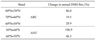
2.2 The simulation methodWe compared the two classes of AGCM outputs: the first state is the control run (Baseline, indicated as B00) with input forcings, anthropogenic and natural sulfur sources representing a contemporary climate (late 20th century) (Fig. 2). The AGCM was initially spun up to 50 years to make sure the model is approaching an equilibrium state (Gabric et al., 2013). The second state is the modified run (indicated as B01), that is after applying DMS flux perturbations in the south and north polar regions according to the 10° latitude bands in Table 1. The maximum perturbation of DMS flux is 106.9% and occurs within the 50°S–60°S band. In both runs (B00 and B01), outputs were obtained by averaging the final 10 years of the simulation. The relative increase in each zonal band is shown in Fig. 1 in Gabric et al. (2013).

|
| Fig.2 Monthly change in DMS vertical integral between baseline (B00) and modified simulations (B01) for the Antarctic (ANT) and Arctic (ARC) |
We consider some of the caveats in the present analysis. Firstly, the modeling assumes that no significant species distribution changes would occur, as the marine food web gradually adapts to warming. However, planktonic populations can respond to ocean variability rather sensitively and quickly (Coello-Camba and Agustí, 2017).
Secondly, any changes to nutrient supply to the surface ocean under warming have not been included explicitly, although these could occur from changes in either ocean upwelling or wind-driven aeolian deposition (Gabric et al., 2004).
The possible future physical changes (such as variation of sea ice melt, wind speed, sea surface temperature, and mixed layer depth (MLD)) can all have large impacts on the DMS flux perturbations applied here. The MLD influences DMS water column concentrations (Simó and Dachs, 2002). Ice melt waters stimulate the growth of phytoplankton biomass (Matrai and Vernet, 1997). The DMS flux is the product of DMS and transfer velocity (related to the wind speed and sea surface temperature) (Liss and Merlivat, 1986; Nightingale et al., 2000).
Moreover, we note that DMS synthesis and emission is the result of whole food-web interactions. Such complex adaptive systems display nonlinearity and multiple feedbacks with future behavior are difficult to predict (Gabric et al., 2004).
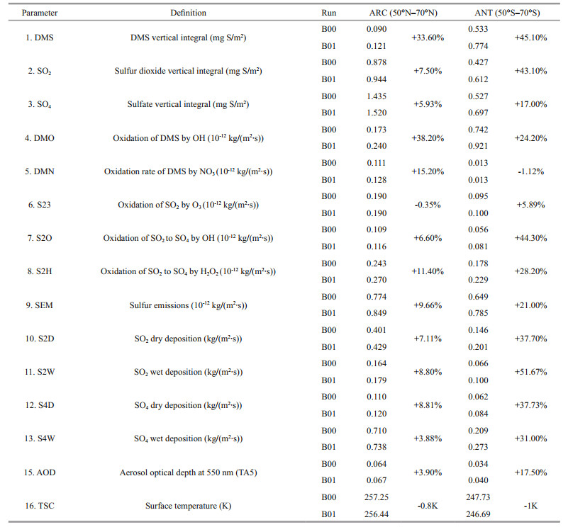
3 RESULTThe monthly means for each model state variable are compared between the baseline (B00) and perturbed simulations (B01) in Table 2 for both Antarctic (ANT) and Arctic (ARC). After perturbation (B01), the DMS vertical integral increases by 45.1% in ANT and increases by 33.6% in ARC. The SO2 vertical integral increases by 43.1% in ANT but only increases by 7.5% in ARC. The much higher simulated increase of DMS flux leads to higher SO2 levels in ANT. Although relevant lower increase rates of DMS and SO2 in ARC, the SO2 profiles (for both B00 and B01) are much higher in ARC (Fig. 3, blue lines). DMS profiles (Fig. 2) in ANT show that it has a maximum in May and minimum in October. Elevated DMS profiles in ANT indicate that there are more biogenic sulfurs emitted in ANT than ARC. SO2 has its peak in spring (February and March) and minimum during summer (July) (Fig. 3).
|

|
| Fig.3 Monthly change in sulfur dioxide vertical integral (SO2) between baseline (B00) and modified simulations (B01) for the ANT and ARC |
The higher spring SO2 in ARC can be affected by Arctic haze that comes mainly from anthropogenic sources of continental aerosols (Shaw, 1995). These aerosols are transported from middle latitude source regions and contribute to the Arctic haze during winter and springtime. These aerosols are primarily composed of sulfate and both directly and indirectly affect Arctic climate (Shaw, 1995; Quinn et al., 2007; Zhao and Garrett, 2015). There is no phenomenon of polar haze in the SH simply because of the absence of anthropogenic pollution near the Antarctic.
The changes in annual mean atmospheric DMS vertical integral in both ARC and ANT are significant. Both the North Atlantic and North Pacific Oceans show a large increase in the DMS vertical integral. The Antarctic Ocean has a significant increase of DMS vertical integral within 50°S–70°S, with peaks along 60°S (not show in figures).
Chen et al. (2018) studied the oxidation of DMS and found that the chemical conversion into SO2 and methane sulfonic acid (MSA) is the key process for the formation and growth of sulfur-containing aerosol and CCN. Their model results indicate that the DMS conversion into SO2 and MSA is 75% and 15%, respectively. The gas-phase oxidation of DMS by OH and NO3 are 91% and 9%, respectively. The dominant gas-phase oxidation pathway of DMS by OH has been noted by numerous researchers (Chen et al., 2000, 2018; Lv et al., 2019; Yan et al., 2020). Yan et al. (2020) found that the conversion ratio of MSA to DMS decreases dramatically as DMS concentration increases when DMS is relatively low. The effect of SST and relative humidity on conversion of DMS to MSA is negligible in the Antarctic Ocean. Our model simulation results show that SO4 increases by 17% in ANT and 5.9% in ARC. Sulfur emissions (SEM) represent the total sulfur emission and is dominated by anthropogenic emissions in ARC but mainly biogenic emissions in ANT. SEM increases by 21% in ANT and increases around 10% in ARC. The maximum of SO2 is in February or March (when Arctic Haze occurs). In ARC, SO4 has a maximum in May. In ANT, SO4 reaches a maximum in the austral summer (December and January). The maximum of SO4 is similar to DMS and about 3–4 months later than SO2 in ARC. The maximum of SEM is generally in summer and has austral summer high in ANT (January) and summer maximum (June) in ARC (Fig. 4, blue and green lines).

|
| Fig.4 Comparison of monthly mean SO4 and SEM for baseline (B00) and modified (B01) simulations for ANT and ARC |
Davis et al. (1998) found that the OH/DMS addition reaction is a major source of DMSO. The OH/DMS addition reaction, as well as follow-on reactions involving OH/DMSO, are a major source of SO2. Preunkert et al. (2008) reported that OH and NO3 are the most efficient atmospheric oxidants of DMS in the Antarctic. They found the lifetime of DMS oxidation by OH is very long in the Antarctic and up to 60 days in May. Hoffmann et al. (2016) indicated that the higher OH concentration arises from reduced ozone depletion by halogens, which enhances the photolysis of O3 as well as OH production. Clouds significantly lower the gas-phase of OH concentrations and modify the prevailing chemistry of the oxidation of DMS and its oxidation products. Hoffmann et al. (2016) also pointed out that during cloudy periods, 78% of DMS is oxidized by O3 to DMSO. During cloud present periods, the overall rate of DMS degradation decreases and the gas-phase DMS concentration increases slightly.
Importantly, the increase rates of oxidation of DMS by hydroxyl radicals (OH) (DMO) and oxidation of DMS by nitrate radicals (NO3) (DMN) are all higher in ARC (38.2% and 15.2% respectively) than ANT (24.2% and decreases -1.12% respectively) (Table 2).
The monthly mean profiles of oxidation of DMS by OH (DMO) all have summer maxima in both polar regions (Fig. 5). The reason could be the OH is most commonly generated by photolysis and DMO reaches maximum in summer period. The maximum of DMO in ANT is higher than the maximum in ARC. The production rate of DMO is higher during November and December, and also higher from January to May in ANT (Fig. 5). However, from September to late October, DMO has decreased tendency from B00 to B01, especially during the austral spring season.

|
| Fig.5 Comparison of monthly mean DMO and DMN for baseline (B00) and modified (B01) simulations for ANT and ARC |
Oxidation of DMS by NO3 (DMN) monthly mean profiles are lower than by OH (DMO) in both polar regions, especially low in ANT (green curve in Fig. 5). The peaks of DMN in ARC are in March and October.
The rates of oxidation of SO2 to SO4 by OH (S2O), oxidation of SO2 by O3 (S23), and oxidation of SO2 to SO4 by H2O2 (S2H) are listed in Table 2. In general, ANT has higher increased rates after DMS flux perturbation (B01 in Table 2). The largest rate of change among the three is S2O (increases by 44.3% in ANT). S23 has a slightly decreased rate in ARC. The profiles of monthly mean of S2O and S23 are shown in Fig. 6. Although there are less increase rates in ARC for B01, the S2O and S23 still have higher monthly mean profiles in ARC (red and blue curves) compare to ANT (purple and green curves). The maximum value of S2O occurs in May (red curves) in ARC and the maximum value of S23 is in September to October in ARC (blue curves). The maximum values of S2O and S23 are in March and January respectively in ANT. The higher profiles in ARC related to the higher SO2 in ARC (Fig. 3). The relevant higher increase rates of S2O are during January to March in ANT (purple curve) and March in ANT for S23 (green curve).

|
| Fig.6 Comparison of monthly mean S2O and S23 for baseline (B00) and modified (B01) simulations for ANT and ARC |
Table 2 shows that SO2 dry deposition (S2D) and SO4 dry deposition (S4D) increase around 37.7% and 7%–8% for ANT and ARC respectively; SO2 wet deposition (S2W) increases more in ANT (reaching to 51.67%) and SO4 wet deposition (S4W) increases by 31% in ANT and increases by 3.88% in ARC. General trends of S2D (Fig. 7, red curves) and S4W in ARC (Fig. 8, blue curves) are especially higher. In ARC, S2D and S2W have their maximum values in February (Fig. 7, red and blue curves) and S4D and S4W have their maximum values in June (Fig. 8, red and blue curves). In ANT, both SO2 and SO4 related dry and wet depositions (S2D, S2W, S4D, and S4W) also have their maxima during the summer months (January or December). SO2 related dry and wet depositions (S2D and S2W) in ANT have highest increase rate in March, which is just after the austral summer (Fig. 7, purple and green curves).

|
| Fig.7 Comparison of monthly mean S2D and S2W for baseline (B00) and modified (B01) simulations for ANT and ARC |

|
| Fig.8 Comparison of monthly mean S4D and S4W for baseline (B00) and modified (B01) simulations for ANT and ARC |
After DMS flux perturbation, AOD increases by 17.5% in ANT compared with 3.9% in ARC (Table 2). Surface temperature (TSC) decreases 1 K in ANT and decrease 0.8 K in ARC. Figure 9 shows monthly mean AOD and TSC (surface temperature) for B00 (solid lines) and B01 (dash lines). In the ARC, maximum AOD occurs in May, and maximum TSC is in July. In ANT, AOD, and TSC all have maxima in summertime (December or January). The obvious increment of AOD from B00 to B01 in ANT are shown in Fig. 9 especially during austral summer (DJF) (the purple lines). The increment rate of AOD during austral summer (DJF) is 23.8%. The differences of annual mean images of AOD between B00 and B01 are shown in Fig. 10. The global mean changes of AOD from B00 to B01 (Fig. 10a) indicate the most significant increase of AOD is within ANT region. The most significant change of AOD in austral summer (DJF) is shown in Fig. 10b. Notice the different scales for the annual mean and summer mean in Fig. 10b.

|
| Fig.9 Comparison of monthly mean AOD and TSC for baseline (B00) and modified (B01) simulations for ANT and ARC |

|
| Fig.10 Aerosol optical depth at 550 nm (AOD) images for the difference (B01-B00) a. global annual mean; b. ANT annual mean and ANT summertime mean (DJF). |
We simulate the impact on atmospheric chemistry of a change in DMS flux in both polar regions: ANT (50°S–70°S) and ARC (65°N–80°N). Our results indicate that there is a noticeable difference between the impacts in the two polar regions. In general, most quantities related to the sulfur cycle show higher rates of change in ANT especially during the austral summer. However, the higher sulfurs mostly appear in ARC. The perturbation on DMS flux leads to an increase in the DMS vertical integral of around 45% in ANT and increase 33.6% in ARC.
Shon et al. (2001) found that the conversion from DMS to SO2 in ANT is as high as 70% or over, giving the lifetime of one day. In Arctic Ocean, sensitivity tests were made by Mungall et al. (2016). They found that DMS sources come from non-marine sources (such as continental air-mass originally from land surfaces and sea ice; snow melts and sea salt aerosols from melt ponds; biomass burning plume) as well as marine source. However, some researchers found the relationship of DMS flux and CCN is rather weak. Woodhouse et al. (2010) pointed out that the sensitivity of CCN to potential future changes in DMS flux is very low. They even suspect the role of DMS in climate regulation is very weak. High concentration of CCN is coincident with strong anthropogenic sources. In high latitude polar oceans, CCN exhibits low concentrations. Quinn and Bates (2011) also suspected the CLAW hypothesis and they ruled out CCN mostly formed by DMS flux which hypothesized by CLAW and pointed out CCN could also formed by sea-salt particles. Liu et al. (2011) discovered that reduced concentrations of H2SO4 due to slower oxidation of SO2 by the OH in winter results in a lower aging rate and thus weaker wet deposition.
Our result shows that the oxidation of SO2 to SO4 by OH (S2O) increases by 44.3% in ANT but only increases by 6.6% in ARC. Sulfur emissions increases by 21% in ANT and increases by 9.7% in ARC. SO4 wet and dry depositions all increases more in ANT (more than 30%) and only a little increase in ARC (less than 10%). The changes in sulfate are relatively smaller than the changes in DMS emissions. AOD increases by 17.5% in ANT and only increases around 4% in ARC. After DMS flux perturbations. Surface temperature (TSC) reduces 1 K in ANT and reduces 0.8 K in ARC.
It is clear, the impact of warming on future DMS flux is model dependent, spatially variable. Numerous researchers confirmed that more contributions of DMS sea-air fluxes are in the polar regions (Gabric et al., 2003, 2004, 2005a, 2010, 2013; Korhonen et al., 2008, 2010; Qu and Gabric, 2010; Qu et al., 2016, 2017). The production of new DMS-derived CCN can take several days. During this time, DMS may be advected large distances; therefore, DMS impacts on aerosol levels are strongly non-local. However, even small changes in CCN may have significant effect on climate in remote unpolluted regions. DMS emissions could exert a more significant influence on a low aerosol concentrated prevailing area, such as the Arctic in summer according to model simulations by Woodhouse et al. (2013). It is also reinforced by reports linking new particle formation events in the polar atmosphere to DMS emission by numerous researchers (Leck and Bigg, 2010; Croft et al., 2016; Park et al., 2017; Kerminen et al., 2018; Jang et al., 2019). Our previous results consistently show the future increase of DMS flux in Barents Sea and Greenland Sea due to ice melting in Arctic Ocean (Qu and Gabric, 2010; Qu et al., 2016, 2017). Our decadal studies suggest that the DMS flux would increase significantly in polar regions during the latter part of the 21st century. The DMS flux perturbations are likely to cause more cooling in surface temperature in the Antarctic and Arctic Oceans due to their relatively unpolluted environment.
5 DATA AVAILABILITY STATEMENTThe datasets generated and/or analyzed during the current study are available from the corresponding author on reasonable request.
6 ACKNOWLEDGMENTWe thank Dr. Leon Rotstayn (CSIRO) who conducted the AGCM runs for our analysis. Special thanks should also go to Nantong University, China, for providing this opportunity of further cooperation between China and Australia. We also gratefully acknowledge the financial assistance of an ASAC Grant from the Australian Antarctic Division for providing research funding for this project.
Bates T S, Lamb B K, Guenther A, Dignon J, Stoiber R E. 1992. Sulfur emissions to the atmosphere from natural sources. Journal of Atmospheric Chemistry, 14(1-4): 315-337.
DOI:10.1007/BF00115242 |
Bopp L, Aumont O, Belviso S, Monfray P. 2003. Potential impact of climate change on marine dimethyl sulfide emissions. Tellus B, 55(1): 11-22.
DOI:10.3402/tellusb.v55i1.16359 |
Charlson R J, Lovelock J E, Andreae M O, Warren S G. 1987. Oceanic phytoplankton, atmospheric sulphur, cloud albedo and climate. Nature, 326(6114): 655-661.
DOI:10.1038/326655a0 |
Chen G, Davis D D, Kasibhatla P, Bandy A R, Thornton D C, Huebert B J, Clarke A D, Blomquist B W. 2000. A study of DMS oxidation in the tropics:comparison of Christmas Island field observations of DMS, SO2, and DMSO with model simulations. Journal of Atmospheric Chemistry, 37(2): 137-160.
DOI:10.1023/A:1006429932403 |
Chen Q J, Sherwen T, Evans M, Alexander B. 2018. DMS oxidation and sulfur aerosol formation in the marine troposphere:a focus on reactive halogen and multiphase chemistry. Atmospheric Chemistry and Physics, 18(18): 13 617-13 637.
DOI:10.5194/acp-18-13617-2018 |
Coello-Camba A, Agustí S. 2017. Thermal thresholds of phytoplankton growth in polar waters and their consequences for a warming polar ocean. Frontiers in Marine Science, 4: 168.
DOI:10.3389/fmars.2017.00168 |
Croft B, Wentworth G R, Martin R V, Leaitch W R, Murphy J G, Murphy B N, Kodros J K, Abbatt J P D, Pierce J R. 2016. Contribution of Arctic seabird-colony ammonia to atmospheric particles and cloud-albedo radiative effect. Nature Communications, 7: 13444.
DOI:10.1038/ncomms13444 |
Davis D, Chen G, Kasibhatla P, Jefferson A, Tanner D, Eisele F, Lenschow D, Neff W, Berresheim H. 1998. DMS oxidation in the Antarctic marine boundary layer:comparison of model simulations and held observations of DMS, DMSO, DMSO2, H2SO4(g), MSA(g), and MSA(p). Journal of Geophysical Research, 103(D1): 1 657-1 678.
DOI:10.1029/97JD03452 |
Feichter J, Kjellström E, Rodhe H, Dentener F, Lelieveldi J, Roelofs G J. 1996. Simulation of the tropospheric sulfur cycle in a global climate model. Atmospheric Environment, 30(10-11): 1 693-1 707.
DOI:10.1016/1352-2310(95)00394-0 |
Gabric A J, Cropp R, Hirst T, Marchant H. 2003. The sensitivity of dimethyl sulfide production to simulated climate change in the Eastern Antarctic Southern Ocean. Tellus B, 55(5): 966-981.
DOI:10.1034/j.1600-0889.2003.00077.x |
Gabric A J, Cropp R A, McTainsh G H, Johnston B M, Butler H, Tilbrook B, Keywood M. 2010. Australian dust storms in 2002-2003 and their impact on Southern Ocean biogeochemistry. Global Biogeochemical Cycles, 24(2): GB2005.
DOI:10.1029/2009GB003541 |
Gabric A J, Matrai P, Jones G, Middleton J. 2018. The nexus between sea ice and polar emissions of marine biogenic aerosols. Bulletin of the American Meteorological Society, 99(1): 61-81.
DOI:10.1175/BAMS-D-16-0254.1 |
Gabric A J, Qu B, Matrai P A, Hirst A C. 2005a. The simulated response of dimethylsulfide production in the Arctic Ocean to global warming. Tellus B, 57(5): 391-403.
DOI:10.3402/tellusb.v57i5.16564 |
Gabric A J, Qu B, Matrai P A, Murphy C, Lu H L, Lin D R, Qian F, Zhao M. 2014. Investigating the coupling between phytoplankton biomass, aerosol optical depth and sea-ice cover in the Greenland Sea. Dynamics of Atmospheres and Oceans, 66: 94-109.
DOI:10.1016/j.dynatmoce.2014.03.001 |
Gabric A J, Qu B, Rotstayn L, Shephard J M. 2013. Global simulations of the impact on contemporary climate of a perturbation to the sea-to-air flux of dimethylsulfide. Australian Meteorology and Oceanographic Journal, 63: 365-376.
DOI:10.22499/2.6303.002 |
Gabric A J, Simó R, Cropp R A, Hirst A C, Dachs J. 2004. Modeling estimates of the global emission of dimethylsulfide under enhanced greenhouse conditions. Global Biogeochemical Cycles, 18(2): GB2014.
DOI:10.1029/2003gb002183 |
Ghahremaninezhad R, Gong W, Galí M, Norman A L, Beagley S R, Akingunola A, Zheng Q, Lupu A, Lizotte M, Levasseur M, Leaitch W R. 2019. Dimethyl sulfide and its role in aerosol formation and growth in the Arctic summer-a modelling study. Atmospheric Chemistry and Physics, 19(23): 14 455-14 476.
DOI:10.5194/acp-19-14455-2019 |
Ghahremaninezhad R, Norman A L, Abbatt J P D, Levasseur M, Thomas J L. 2016. Biogenic, anthropogenic and sea salt sulfate size-segregated aerosols in the Arctic summer. Atmospheric Chemistry and Physics, 16(8): 5 191-5 202.
DOI:10.5194/acp-16-5191-2016 |
Gordon H B, O'Farrell S P. 1997. Transient climate change in the CSIRO coupled model with dynamic sea ice. Monthly Weather Review, 125(5): 875-907.
DOI:10.1175/1520-0493(1997)125<0875:TCCITC>2.0.CO;2 |
Gordon H B, Rotstayn L D, McGregor J L, Dix M R, Kowalczyk E A, O'Farrell S P, Waterman L J, Hirst A C, Wilson S G, Collier M A, Watterson I G, Elliott T I. 2002.The CSIRO Mk3 Climate System Model. CSIRO Atmospheric Research Technical Paper No. 60.
|
Hoffmann E H, Tilgner A, Schrödner R, Bräuer P, Wolke R, Herrmann H. 2016. An advanced modeling study on the impacts and atmospheric implications of multiphase dimethyl sulfide chemistry. Proceedings of the National Academy of Sciences of the United States of America, 113(42): 11 776-11 781.
DOI:10.1073/pnas.1606320113 |
Hunt B G, Davies H L. 1997. Mechanism of multidecadal climatic variability in a global climatic model. International Journal of Climatology, 17(6): 565-580.
DOI:10.1002/(SICI)1097-0088(199705)17:6<565::AID-JOC172>3.0.CO;2-6 |
Jang E, Park K T, Yoon Y J, Kim T W, Hong S B, Becagli S, Traversi R, Kim J, Gim Y. 2019. New particle formation events observed at the King Sejong Station, Antarctic Peninsula-Part 2:link with the oceanic biological activities. Atmospheric Chemistry and Physics, 19(11): 7 595-7 608.
DOI:10.5194/acp-19-7595-2019 |
Jung C H, Yoon Y J, Kang H J, Gim Y, Lee B Y, Ström J, Krejci R, Tunved P. 2018. The seasonal characteristics of cloud condensation nuclei (CCN) in the arctic lower troposphere. Tellus B:Chemical and Physical Meteorology, 70(1): 1-13.
DOI:10.1080/16000889.2018.1513291 |
Karl M, Gross A, Leck C, Pirjola L. 2007. Intercomparison of dimethylsulfide oxidation mechanisms for the marine boundary layer:gaseous and particulate sulfur constituents. Journal of Geophysical Research:Atmospheres, 112(D15): D15304.
DOI:10.1029/2006JD007914 |
Kerminen V M, Chen X M, Vakkari V, Petäjä T, Kulmala M, Bianchi F. 2018. Atmospheric new particle formation and growth:review of field observations. Environmental Research Letters, 13(10): 103003.
DOI:10.1088/1748-9326/aadf3c |
Kloster S, Six K D, Feichter J, Maier-Reimer E, Roeckner E, Wetzel P, Stier P, Esch M. 2007. Response of dimethylsulfide (DMS) in the ocean and atmosphere to global warming. Journal of Geophysical Research, 112(G3): G03005.
DOI:10.1029/2006JG000224 |
Korhonen H, Carslaw K S, Forster P M, Mikkonen S, Gordon N D, Kokkola H. 2010. Aerosol climate feedback due to decadal increases in Southern Hemisphere wind speeds. Geophysical Research Letters, 37(2): L02805.
DOI:10.1029/2009gl041320 |
Korhonen H, Carslaw K S, Spracklen D V, Mann G W, Woodhouse M T. 2008. Influence of oceanic dimethyl sulfide emissions on cloud condensation nuclei concentrations and seasonality over the remote Southern Hemisphere oceans:a global model study. Journal of Geophysical Research:Atmospheres, 113(D15): D15204.
DOI:10.1029/2007JD009718 |
Leck C, Bigg E K. 2010. New particle formation of marine biological origin. Aerosol Science and Technology, 44(7): 570-577.
DOI:10.1080/02786826.2010.481222 |
Liss P S, Merlivat L. 1986. Air-sea gas exchange rates: introduction and synthesis. In: Buat-Ménard P ed. The Role of Air-Sea Exchange in Geochemical Cycling.NATO ASI Series (Series C: Mathematical and Physical Sciences), vol. 185. Springer, Dordrecht. p.113-127, https://doi.org/10.1007/978-94-009-4738-2_5.
|
Liu J F, Fan S M, Horowitz L W, Levy H Ⅱ. 2011. Evaluation of factors controlling long-range transport of black carbon to the Arctic. Journal of Geophysical Research:Atmospheres, 116(D4): D04307.
DOI:10.1029/2010jd015145 |
Lohmann U, Feichter J, Chuang C C, Penner J E. 1999. Prediction of the number of cloud droplets in the ECHAM GCM. Journal of Geophysical Research:Atmospheres, 104(D8): 9 169-9 198.
DOI:10.1029/1999JD900046 |
Lovelock J E, Maggs R J, Rasmussen R A. 1972. Atmospheric dimethyl sulphide and the natural sulphur cycle. Nature, 237(5356): 452-453.
DOI:10.1038/237452a0 |
Lv G C, Zhang C X, Sun X M. 2019. Understanding the oxidation mechanism of methanesulfinic acid by ozone in the atmosphere. Scientific Reports, 9(1): 322.
DOI:10.1038/s41598-018-36405-0 |
Malin G. 1997. Sulphur, climate and the microbial maze. Nature, 387(6636): 857-858.
DOI:10.1038/43075 |
Matrai P A, Vernet M. 1997. Dynamics of the vernal bloom in the marginal ice zone of the Barents Sea:dimethyl sulfide and dimethylsulfoniopropionate budgets. Journal of Geophysical Research:Oceans, 102(C10): 22 965-22 979.
DOI:10.1029/96JC03870 |
Mungall E L, Croft B, Lizotte M, Thomas J L, Murphy J G, Levasseur M, Martin R V, Wentzell J J B, Liggio J, Abbatt J P D. 2016. Dimethyl sulfide in the summertime Arctic atmosphere:measurements and source sensitivity simulations. Atmospheric Chemistry and Physics, 16(11): 6 665-6 680.
DOI:10.5194/acp-16-6665-2016 |
Nightingale P D, Malin G, Law C S, Watson A J, Liss P S, Liddicoat M I, Boutin J, Upstill-Goddard R C. 2000. In situ evaluation of air-sea gas exchange parameterizations using novel conservative and volatile tracers. Global Biogeochemical Cycles, 14(1): 373-387.
DOI:10.1029/1999GB900091 |
O'Farrell S P. 1998. Investigation of the dynamic sea ice component of a coupled atmosphere-sea ice general circulation model. Journal of Geophysical Research:Oceans, 103(C8): 15 751-15 782.
DOI:10.1029/98JC00815 |
Park K T, Jang S, Lee K, Yoon Y J, Kim M S, Park K, Cho H J, Kang J H, Udisti R, Lee B Y, Shin K H. 2017. Observational evidence for the formation of DMS-derived aerosols during Arctic phytoplankton blooms. Atmospheric Chemistry and Physics, 17(15): 9 665-9 675.
DOI:10.5194/acp-17-9665-2017 |
Preunkert S, Jourdain B, Legrand M, Udisti R, Becagli S, Cerri O. 2008. Seasonality of sulfur species (dimethyl sulfide, sulfate, and methanesulfonate) in Antarctica:inland versus coastal regions. Journal of Geophysical Research:Atmospheres, 113(D15): D15302.
DOI:10.1029/2008JD009937 |
Qu B, Gabric A J. 2010. Using genetic algorithms to calibrate a dimethylsulfide production model in the Arctic Ocean. Chinese Journal of Oceanology and Limnology, 28(1): 573-582.
DOI:10.1007/s00343-010-9062-x |
Qu B, Gabric A J, Jiang L, Li C. 2020. Comparison between early and late 21st C phytoplankton biomass and dimethylsulfide flux in the subantarctic southern ocean. Journal of Ocean University of China, 19(1): 151-160.
DOI:10.1007/s11802-020-4235-5 |
Qu B, Gabric A J, Lu H L, Lin D R. 2014. Spike in phytoplankton biomass in Greenland Sea during 2009 and the correlations among chlorophyll-a, aerosol optical depth and ice cover. Chinese Journal of Oceanology and Limnology, 32(2): 241-254.
DOI:10.1007/s00343-014-3141-3 |
Qu B, Gabric A J, Zeng M F, Lu Z F. 2016. Dimethylsulfide model calibration in the Barents Sea using a genetic algorithm and neural network. Environmental Chemistry, 13(2): 413-424.
DOI:10.1071/EN14264 |
Qu B, Gabric A J, Zeng M F, Xi J J, Jiang L M, Zhao L. 2017. Dimethylsulfide model calibration and parametric sensitivity analysis for the Greenland Sea. Polar Science, 13: 13-22.
DOI:10.1016/j.polar.2017.07.001 |
Qu B, Gabric A J, Zhao L, Sun W J, Li H H, Gu P J, Jiang L M, Zeng M F. 2018. The relationships among aerosol optical depth, ice, phytoplankton and dimethylsulfide and the implication for future climate in the Greenland Sea. Acta Oceanologica Sinica, 37(5): 13-21.
DOI:10.1007/s13131-018-1210-8 |
Quinn P K, Bates T S. 2011. The case against climate regulation via oceanic phytoplankton sulphur emissions. Nature, 480(7375): 51-56.
DOI:10.1038/nature10580 |
Quinn P K, Coffman D J, Johnson J E, Upchurch L M, Bates T S. 2017. Small fraction of marine cloud condensation nuclei made up of sea spray aerosol. Nature Geoscience, 10: 674-679.
DOI:10.1038/ngeo3003 |
Quinn P K, Shaw G, Andrews E, Dutton E G, Ruoho-Airola T, Gong S L. 2007. Arctic haze:current trends and knowledge gaps. Tellus B, 59(1): 99-114.
DOI:10.1111/j.1600-0889.2006.00236.x |
Rotstayn L D, Lohmann U. 2002. Simulation of the tropospheric sulfur cycle in a global model with a physically based cloud scheme. Journal of Geophysical Research:Atmospheres, 107(D21): AAC 20-21-AAC 20-21.
DOI:10.1029/2002jd002128 |
Rotstayn L D, Penner J E. 2001. Indirect aerosol forcing, quasi forcing, and climate response. Journal of Climate, 14(13): 2 960-2 975.
DOI:10.1175/1520-0442(2001)014<2960:IAFQFA>2.0.CO;2 |
Shaw G E. 1995. The arctic haze phenomenon. Bulletin of the American Meteorological Society, 76(12): 2 403-2 414.
DOI:10.1175/1520-0477(1995)076<2403:TAHP>2.0.CO;2 |
Shon Z H, Davis D, Chen G, Grodzinsky G, Bandy A, Thornton D, Sandholm S, Bradshaw J, Stickel R, Chameides W, Kok G, Russell L, Mauldin L, Tanner D, Eisele F. 2001. Evaluation of the DMS flux and its conversion to SO2 over the southern ocean. Atmospheric Environment, 35(1): 159-172.
DOI:10.1016/S1352-2310(00)00166-7 |
Simó R, Dachs J. 2002. Global ocean emission of dimethylsulfide predicted from biogeophysical data. Global Biogeochemical Cycles, 16(4): 26-1-26-10.
DOI:10.1029/2001GB001829 |
Vallina S M, Simó R, Gassó S. 2006. What controls CCN seasonality in the Southern Ocean? A statistical analysis based on satellite-derived chlorophyll and CCN and model-estimated OH radical and rainfall. Global Biogeochemical Cycles, 20(1): GB1014.
DOI:10.1029/2005GB002597 |
Vallina S M, Simó R, Gassó S, de Boyer-Montégut C, Del Río E, Jurado E, Dachs J. 2007. Analysis of a potential "solar radiation dose-dimethylsulfide-cloud condensation nuclei" link from globally mapped seasonal correlations. Global Biogeochemical Cycles, 21(2): GB2004.
DOI:10.1029/2006GB002787 |
Woodhouse M T, Carslaw K S, Mann G W, Vallina S M, Vogt M, Halloran P R, Boucher O. 2010. Low sensitivity of cloud condensation nuclei to changes in the sea-air flux of dimethyl-sulphide. Atmospheric Chemistry and Physics, 10(16): 7 545-7 559.
DOI:10.5194/acp-10-7545-2010 |
Woodhouse M T, Mann G W, Carslaw K S, Boucher O. 2013. Sensitivity of cloud condensation nuclei to regional changes in dimethyl-sulphide emissions. Atmospheric Chemistry and Physics, 13(5): 2 723-2 733.
DOI:10.5194/acp-13-2723-2013 |
Yan J P, Zhang M M, Jung J, Lin Q, Zhao S H, Xu S Q, Chen L Q. 2020. Influence on the conversion of DMS to MSA and SO42- in the Southern Ocean, Antarctica. Atmospheric Environment, 233: 117611.
DOI:10.1016/j.atmosenv.2020.117611 |
Zhao C F, Garrett T J. 2015. Effects of Arctic haze on surface cloud radiative forcing. Geophysical Research Letters, 42(2): 557-564.
DOI:10.1002/2014GL062015 |