 2021, Vol. 39
Institute of Oceanology, Chinese Academy of Sciences
Article Information
- LIM Joon Hai, LEE Choon Weng, BONG Chui Wei
- Investigating factors driving phytoplankton growth and grazing loss rates in waters around Peninsular Malaysia
- Journal of Oceanology and Limnology, 39(1): 148-159
- http://dx.doi.org/10.1007/s00343-020-9227-1
Article History
- Received Sep. 24, 2019
- accepted in principle Dec. 17, 2019
- accepted for publication Mar. 8, 2020


2 Institute of Ocean and Earth Sciences, University of Malaya, Kuala Lumpur 50603, Malaysia;
3 Institute for Advanced Studies, University of Malaya, Kuala Lumpur 50603, Malaysia
In the oceans, primary production is mainly carried out by phytoplankton (Duarte and Cebrián, 1996; Field et al., 1998), and phytoplankton biomass that is produced is transferred to higher trophic level via grazing (Vargas et al., 2007; Selph et al., 2016). Across different regions, microzooplankton grazing accounts for an estimated 44% to 79% of daily primary production (Schmoker et al., 2013). Phytoplankton production not grazed is either lost through horizontal export or sinking (Turner, 2002; Stukel et al., 2011). As primary production and grazing loss rates are affected by different environmental drivers (Boyce et al., 2010; LópezUrrutia and Morán, 2015; Zhang et al., 2018), their values are distributed over a wide range and are sitespecific. It is important to measure these biological processes as the balance between both primary production and grazing rates affects the distribution of primary producers (Zheng et al., 2015; Cermeño et al., 2016).
In a cross-compilation study of 110 datasets by Schmoker et al. (2013), only 24% were from tropical waters. Data from Sunda Shelf were clearly lacking even though two additional studies were published from the Sunda Shelf waters i.e. Strait of Malacca (Lim et al., 2015, 2018) and Strait of Singapore (Schmoker et al., 2016). Sunda Shelf waters are highly productive tropical waters (Ooi et al., 2013), and clear differences in terms of eutrophication exist in waters around Peninsular Malaysia (Lim et al., 2018).
Although temperature is an important environmental driver of biological processes (Boyce et al., 2010), in tropical waters where temperatures are stable, most biological processes are already functioning at near optimum (Pomeroy and Wiebe, 2001). Therefore, the balance between primary production and grazing loss rates in these waters are primarily determined by the productivity or trophic state of the waters as grazing loss is reported to be higher in productive waters (Schmoker et al., 2013). In this study, we hope to determine whether the statement holds true by adopting the Landry and Hassett (1982) dilution method to measure concurrent phytoplankton growth and grazing loss rate. Despite the possible limitation of this approach, i.e. nutrient limitation, grazing saturation and non-linear response (Ayukai, 1996; Paterson et al., 2008; Schmoker et al., 2016), the rates obtained via this method have generally been comparable to the more common light-dark dissolved oxygen and 14C uptake methods (Landry et al., 2011; Lim et al., 2015; Selph et al., 2016).
In this study, we measured phytoplankton growth and grazing loss rates in waters northeast of Peninsular Malaysia (BMRS), and then analysed these rates from waters around Peninsular Malaysia: west of Peninsular Malaysia i.e. Port Klang (PK) and Port Dickson (PD) (Lim et al., 2015); northwest (NW) and southeast (SE) of Peninsular Malaysia (submitted); and south of Peninsular Malaysia i.e. Strait of Singapore (SS) (Schmoker et al., 2016). In general, NW and SE stations were shelf waters located >5 km away from the shoreline whereas BMRS and PD were stations located next to sandy beaches. PK was at Klang River estuary and SS was an enclosed bay south of Singapore. For nearshore habitats such as BMRS, PD, PK and SS, they are commonly influenced by semidiurnal tide where two episodes of equally high and low waters are recorded each day.
At present, we aim to address the following questions: What are the growth and grazing loss rate of primary producers in the northeast coast of Peninsular Malaysia and can the differences in phytoplankton growth and grazing loss rate across different habitats around Peninsular Malaysia be attributed to its trophic states? Other than filling in an obvious data gap, the short-term sampling at BMRS would also allow us to better understand the fluctuation of phytoplankton growth and grazing loss rates throughout the day. These short-term data are unavailable from published reports in this region (Lim et al., 2015; Schmoker et al., 2016). As primary production and grazing loss rates can respond rapidly to environmental change (Goes et al., 2016), the results obtained here could also direct us on possible long-term research strategies.
2 MATERIAL AND METHOD 2.1 Sampling and physiochemical parametersSampling was carried out at Bachok Marine Research Station (BMRS) (6°00′N, 102°25′E), located northeast coast of Peninsular Malaysia (Fig. 1). Twelve samplings were carried out over a three-day period where about 10-L sample was collected every time. Temperature, salinity (YSI Pro- 30, USA), and pH (Metrohm 827, Switzerland) were measured in-situ whereas dissolved oxygen (DO) concentration was determined via Winkler titration method (Grasshoff et al., 1999).

|
| Fig.1 The study area and sampling locations The filled circle: the BMRS (6°00′N, 102°25′E) at the northeast coast of Peninsular Malaysia; filled triangles: the locations where data from the northwest (NW) and southeast (SE) coast of Peninsular Malaysia (submitted), Port Dickson (PD), Port Klang (PK) (Lim et al., 2015) and Strait of Singapore (SS) (Schmoker et al., 2016) were compiled for the systematic review. |
Seawater sample was filtered through glass fiber filters (GF/F) that were pre-combusted at 500 ℃ for 3 h. The filtrate was then kept at -20 ℃ before dissolved inorganic nutrient analyses (ammonium: NH4; phosphate: PO4; nitrate+nitrite: NO3+NO2; and silicate: SiO4) whereas the filters were kept for chlorophyll a (chl a) and total suspended solid (TSS). Dissolved inorganic nutrients were measured by the colorimetric method with a spectrophotometer (Hitachi U-1800, Japan) (Parsons et al., 1984). NH4 was measured by the blue indophenol method whereas NO3 was reduced to NO2 with a cadmium reduction column before NO3+NO2 was detected as pink diazo compound. For PO4, it was determined through the molybdenum blue method whereas for SiO4, it was first reduced to molybdosilicic acid before its concentration was determined by the molybdenum blue method. TSS was measured by gravimetry method as the net weight increase of the filter after drying at 50 ℃ for seven days. The same filter was later combusted at 500 ℃ for 3 h and the weight loss was calculated as particulate organic matter (POM).
Chlorophyll a retained on the precombusted GF/F was extracted in 90% (v/v) ice-cold acetone at -20 ℃ for approximately 16 h. The fluorescence intensity was then detected at the excitation/emission wavelength of 440/680 nm with a spectrofluorometer (Perkin Elmer LS55 spectrofluorometer, USA). Standardization was carried out with a commercially available chl a standard (Sigma-Aldrich, USA) (Lohrenz et al., 2003). Seawater sample was also passed through the 2-μm and 20-μm (pore size) polycarbonate membrane filters, and chl a in the filtrate as collected on the GF/F filters represented the < 2-μm and < 20-μm fraction, respectively. The >20-μm fraction was calculated as the difference between total chl-a and the < 20-μm fraction whereas the 2–20-μm fraction was calculated as the difference between the < 20-μm and the < 2-μm (Arin et al., 2002).
2.2 Phytoplankton production and grazing loss rateIn the Landry and Hassett (1982) dilution method, seawater sample was filtered through a 0.2-μm filter to prepare particle-free seawater. The particle-free seawater was then used to dilute the sample to 0.2, 0.4, 0.6, 0.8, and 1.0-strength (or undiluted) microcosms. These microcosms were then incubated under 12 h light (340 μmol/(m2·s)): 12 h dark photoperiod at in-situ temperature. The increase in chl-a concentration for each fraction (μi) was calculated as μi=ln chl at–ln chl a0, where chl a0 was the initial chl-a concentration and chl at was the chl-a concentration at the end of the incubation. The μi for each microcosm was then plotted against its dilution factor, and a linear regression analysis was carried out. From the linear regression slope, the y-axis intercept was measured as μ whereas the gradient of the slope was measured as g. In this study, g was total grazing as we did not distinguish between micro- and meso-zooplankton grazing. However, it is generally accepted that microzooplankton grazing is the major factor for the loss of primary producers (Calbet and Landry, 2004; Schmoker et al., 2013).
2.3 Systematic review of waters around Peninsular MalaysiaIn order to understand the drivers for phytoplankton growth and loss rates in waters around Peninsular Malaysia, we carried out a systematic review of published and available data from the NW (n=18) and SE (n=24) coast of Peninsular Malaysia (submitted), PD (n=21), PK (n=19) (Lim et al., 2015) and SS (n=18) (Schmoker et al., 2016). For each station, the trophic state index (TSI) was calculated according to Carlson (1977) by the following equations:
TSI=60–14.41 ln(Secchi depth, m),
TSI=9.81 ln(chl a, μg/L)+30.6.
The average TSI values were then used to characterize these habitats into oligotrophic (TSI < 40), mesotrophic (TSI=40 to 50), and eutrophic (TSI>50) waters.
2.4 Statistical analysisAll values were reported as mean±standard deviation unless otherwise stated. Least-square linear regression analysis was carried out for each dilution experiment whereas analysis of variance and Tukey's test were used to compare values. Correlation analysis was used to show the relationships between the different parameters measured. For statistical analyses, the software PAST Version 2.17c (Hammer et al., 2001) was used.
3 RESULT 3.1 Environmental parametersThe environmental parameters measured at BMRS are shown in Table 1. The surface seawater temperature, salinity, DO and pH observed were relatively similar throughout the sampling period (P > 0.05), and ranged from 28.6 to 31.1 ℃, 27 to 30, 214 to 329 μmol/L and 8.04 to 8.11, respectively. For TSS, the concentration varied from 103 to 156 mg/L, whereas for POM, the concentration fluctuated from 18 to 25 mg/L and represented 14% to 19% of TSS. POM was also higher on the first day of sampling relative to the second and third day (F=9.756, df=5, P < 0.05).
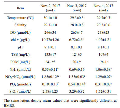
In term of nutrients, dissolved inorganic nitrogen (DIN=NH4+NO3+NO2) ranged from 1.89 to 2.75 μmol/L throughout the monitoring period at BMRS. Among the nitrogen species measured, NH4 and NO3+NO2 fluctuated from 0.21 to 1.38 μmol/L and 1.24 to 2.02 μmol/L (Table 1), respectively with NO3+NO2 contributing 50% to 83% of the fluctuation in DIN. NH4 was significantly different between the first and third day (F=11.38, df=5, P < 0.01), whereas NO3+NO2 was higher in the first than the second and third day of sampling (F=11.61, df=4, P < 0.05). On the other hand, PO4 and SiO4 at BMRS varied from 0.05 to 0.71 μmol/L and 1.50 to 4.39 μmol/L, respectively. On average, PO4 was significant higher on the second day of sampling (F=7.534, df=6, P < 0.05), whereas SiO4 was not different throughout the observation period (P > 0.05).
In this study, total chl-a concentration varied over two-fold at BRMS from 2.90 to 15.78 μg/L. The average total chl-a concentration was however not significantly different throughout the observation period (P > 0.05) (Table 1). From the size-fractionation of chl-a experiment, we found that the dominant fraction was the 2 to 20 μm (50±11)%, followed by the >20-μm fraction (48±12)% and the < 2-μm (2±2)% fractions. Through correlation analysis, the >20-μm fraction could have explicated (74±2)% (F=998, df=11, P < 0.001) of the fluctuation in total chl a, whereas the 2–20-μm fraction could have elucidated only (26±2)% (F=128, df=11, P < 0.001) of the variation in total chl a. The < 2-μm fraction was a minor component and independent of total chl a (P > 0.05).
3.2 Phytoplankton growth and grazing loss ratesOn all occasions, statistically significant regression slopes were obtained but one point (the undiluted fraction at 6 PM, Nov. 3, 2017) was removed (Fig. 2). At BMRS, μ fluctuated daily from 1.02 to 1.58/d (coefficient of variation, CV=14%), whereas g varied over a wider range from 0.07 to 0.88/d (CV=62%). Both μ (P=0.73) and g (P=0.25) were not significantly different throughout the short-term monitoring at BMRS. Among the different chl-a size fractions, changes were apparent after the 24-h incubation. The >20-μm size fraction increased in proportion whereas the < 2-μm size fraction decreased to near undetectable levels.

|
| Fig.2 Linear regression analysis for all the incubation experiments carried out at BMRS The solid line represents regression line throughout the incubation period, and the linear regression equation is also shown as y=mx+b. Filled symbol was an outlier that was not included in the linear regression analysis. |
The environmental parameters for the different habitats are shown in Table 2. The average temperature at BMRS (29.6±0.7 ℃) was lower than at NW (30.7±0.7 ℃) (F=6.288, df=45, P < 0.001), whereas salinity was higher at BMRS (28.9±1.0) than at PK (28.9±1.0) (F=20, df=46, P < 0.001). On average, Secchi depth (0.3±0.1 m) was also lower at BMRS than at NW (9.41±3.37 m), SE (6.83±2.37 m) and SS (3.50±0.71 m) (F=78.34, df=9.63, P < 0.001). In term of dissolved inorganic nutrients, NH4, PO4 and SiO4 were generally lower at BMRS than at PK (F>9.23, df>40, P < 0.001), except for NO3 where the concentration was lower at BMRS (1.31±0.18 μmol/L) than PK (5.69±3.01 μmol/L) and SS (6.09± 9.10 μmol/L) (F=21.79, df=48, P < 0.001). Likewise, the estimated total phosphorus was about three times lower at BMRS (1.49±0.52 μmol/L) than at PK (4.07±3.70 μmol/L) (F=10.68, df=54, P < 0.001).

|
In term of total chl a, the concentration across different habitats typically ranged from 0.20 to 33.56 μg/L. On average, chl a was higher at BMRS (7.17±3.94 μg/L) than at PD (2.31±0.70 μg/L), NW (0.75±0.57 μg/L) and SE (0.72±0.32 μg/L) stations (F=26.73, df=41, P < 0.001) (Fig. 3). From the TSI value, stations at the NW (27±6) and SE (30±4) coast of Peninsular Malaysia represented oligotrophic habitats, PD (49±4) and SS (57±5) were mesotrophic habitats whereas BMRS (63±3) and PK (52±6) were eutrophic habitats. Average μ was higher at BMRS (1.34±0.19/d) than other coastal water stations i.e. NW (0.46±0.20/d), SE (0.55±0.26/d), PD (0.52±0.25/d), SS (0.67±0.53/d), and PK (0.61±0.19/d) (F (5, 106)=34.4, P < 0.001) (Fig. 3). In contrast, g at BMRS (0.44±0.27/d) was not different relative to other stations at NW, SE, PD, SS, and PK that averaged 0.41±0.22/d, 0.37±0.22/d, 0.53±0.23/d, 0.40±0.21/d, and 0.54±0.18/d, respectively (Fig. 3).

|
| Fig.3 Box-and-whisker plots showing the range and median of in-situ chl a (μg/L), phytoplankton growth rate (μ, /d), grazing loss rate (g, /d) and grazing pressure measured at BMRS, northwest (NW) and southeast (SE) coast of Peninsular Malaysia, Port Dickson (PD), stations at the Strait of Singapore (SS) and Port Klang (PK) The same letters denote mean values that were significantly different to BMRS. |
The temperature, salinity and pH observed at BMRS were high and constant (Table 2), typical of coastal waters around Peninsular Malaysia (You et al., 2016; Lim et al., 2018). For DO, the concentration observed at BMRS was generally at healthy levels (>200 μmol/L), and not below the 63 μmol/L consensus concentration for hypoxia (Rabalais et al., 2002). TSS measured at BMRS was also similar to other nearshore coastal waters (≥100 mg/L; Bong and Lee, 2008), and was mostly non-biogenic as POM was ≤19% of TSS. BMRS was characterized as eutrophic system, primarily due to the lower Secchi depth and higher total chl-a concentration observed (Fig. 3) (Lim et al., 2015, 2018). As the sampling was not carried out during the possible upwelling period (June to September) (Syafrina et al., 2015; Suratman et al., 2017), the variation in Secchi depth and chl a were more likely influenced by nearby river output and nearshore physical processes (Shaari and Mustapha, 2017; Suratman et al., 2017; Lim et al., 2018). In addition, size-fractionation of chl a also concurred with other tropical studies where ≥52% of primary producers were >2 μm (Jagadeesan et al., 2017; Madhu et al., 2017).
4.2 Phytoplankton growth and grazing in BMRSAt BMRS, statistically significant linear regression slopes were obtained on all occasions, suggesting that nutrient was generally not limiting phytoplankton growth (Ayukai, 1996; Paterson et al., 2008). Through correlation analysis, we found that μ at BMRS was independent of temperature whereas g correlated with temperature (R2=0.464, df=11, P < 0.01). Although temperature observed at BMRS varied within a narrow range (≤2.5 ℃), the dependency of g could be due to the intrinsic control of grazers through their metabolic rate or extrinsic control that alter the predator-prey encounter rates (Chen et al., 2012; Caron and Hutchins, 2013; López-Urrutia and Morán, 2015; Zhang et al., 2018). We also have evidence that temperature played an important role in regulating different microbial processes in this region (Lee et al., 2009, 2013). In addition, we also found that g at BMRS was significantly correlated with the initial chl-a concentration, specifically the 2–20-μm and >20-μm fractions (Fig. 4). When we compared the regression slopes, g was clearly more dependent on the 2–20-μm fraction of chl a (F=12.27, df=22, P < 0.01). This observation was common as the 2–20-μm fraction of phytoplankton are the basic prey for the main grazers i.e. microzooplankton (>20 μm), accounting for 44% to 79% of g (Schmoker et al., 2013).

|
| Fig.4 Correlation analysis between phytoplankton growth rate (μ, /d) and grazing loss rate (g, /d) to size-fractionation of chl a at BMRS The regression line represents significant correlation. |
In this study, g correlated with μ at BMRS (R2=0.349, df=11, P < 0.05), and reflected the predatorprey coupling that is often observed (Calbet and Landry, 2004; Schmoker et al., 2013; Lim et al., 2015). The relationship between g and μ at BMRS could be expressed via the following linear regression equation: g=0.837μ–0.685 (F=5.350, df=11, P < 0.05). From the equation, g could have accounted for 35% of the fluctuation in μ. The grazing pressure (g/μ) which estimates the fraction of primary production being grazed upon ranged from 0.07 to 0.63 (0.31±0.18) and was always below unity (< 1), suggesting that primary production at BMRS was able to sustain the marine food web. The high chl-a concentration at BMRS was more likely influenced by external sources rather than localized production as the difference in intrinsic phytoplankton growth and grazing loss rate did not reflect in-situ chl a.
4.3 Systematic review of waters around Peninsular MalaysiaIn this study, an extensive range of μ and g by the dilution method (Landry and Hassett, 1982) were compiled from different coastal waters around Peninsular Malaysia. From the rate measurement, we showed that μ was significantly higher at BMRS whereas g was relatively constant throughout the waters of Peninsular Malaysia (Fig. 5). In order to determine the possible environmental factors that drive μ, these data were clustered according to their TSI value (Table 2).

|
| Fig.5 Correlation between chl a (μg/L) and phytoplankton growth rate (μ, /d) for oligotrophic, mesotrophic and eutrophic waters around Peninsular Malaysia The regression line represents significant correlation. Filled symbol were outlier that were excluded from the linear regression analysis. |
For oligotrophic waters, μ was inversely correlated to temperature and suggested that an increasing temperature could have a negative impact on μ (R2=0.240, df=41, P < 0.001). For mesotrophic and eutrophic waters, we found that μ was significantly correlated to chl a (Fig. 5). However, the relationship was only significant at < 9-μg/L chl a (R2=0.337, df=32, P < 0.001) for mesotrophic waters and < 16-μg/L chl a (R2=0.384, df=28, P < 0.001) for eutrophic waters (Fig. 5). The concentration of chl a beyond this threshold was excluded as they are considered outliers (mean±2×standard deviation). Although the abundant nutrients in mesotrophic and eutrophic waters may have complicated this relationship (Yoshiyama and Sharp, 2006; Cloern, 2017; Zhang et al., 2018), the dissolved inorganic nutrients were all independent of μ even in the oligotrophic waters of NW and SE stations (P > 0.05). Our observations seemed to suggest that there was no nutrient limitation in these waters (Lim et al., 2015; Shaari and Mustapha, 2017). The correlation between chl-a concentration and μ could either reflect chl a-driven phytoplankton growth or phytoplankton growth stimulating chl a (Laws et al., 1984; Ning et al., 1988; Tada et al., 2001) in these waters. In this study, we were unable to determine the effect of light on μ because of incomplete data, nonetheless the impact would likely be minimal as all samples were collected from surface (< 1 m in depth) where light intensity is naturally higher (Chavez, 1989).
Regardless of the trophic state, we observed significant coupling between g and μ at every station. Their relationships are as follows: NW: g=0.704 μ+ 0.084 (F=11.8, df=17, P < 0.01); SE: g=0.661 μ+0.006 (F=40.6, df=23, P < 0.001); PD: g=0.679 μ+0.182 (F=25.2, df=20, P < 0.001); SS: g=0.191 μ+0.274 (F=4.86, df=17, P < 0.05); PK: g=0.499 μ+0.237 (F=6.18, df=18, P < 0.05) (Fig. 6). The g/μ slope at NW, SE, PD, SS, and PK accounted for 70%, 66%, 68%, 19%, and 50% of phytoplankton production, respectively. These observations suggested that g was generally an important loss process for u, except at SS when the dependency was lower than the 44% to 79% cross-compilation study by Schmoker et al. (2013). Despite the slope was significantly different (F (5, 105)=3.94, P < 0.01), the average grazing pressure (g/μ) was only lower at BMRS than NW, PD and PK (F (5, 106)=19.4, P < 0.01) (Fig. 3). As there were no long-term measurement of μ and g in this region (≥5 years), all the data in this study were clustered together into four different seasons consisted of northeast (Nov. to Feb.), southwest (May to Aug.) and two shorter inter-monsoons (Mar. to Apr. and Sep. to Oct.) (Syafrina et al., 2015) to determine the possible seasonal effect on g/μ. We found no significant difference for g/μ (P > 0.05), and thus concluded the seasonal impact on g/μ would likely be minimal.

|
| Fig.6 Correlation analyses between grazing loss rate (g, /d) and phytoplankton growth rate (μ, /d) across different habitats around Peninsular Malaysia Solid lines represent significant relationship whereas broken line was 1: 1 ratio. |
Although the composition of organism was not observed, it may play a significant role in regulating the relationship between g and μ across different habitats. For example, the lower dependency of g on μ at SS could be due to the long residence time (about one year) as it was an enclosed bay (Schmoker et al., 2016). As a result, it could have influenced the abundance, food quality, species composition and encounter rates that in turn affected the habitat specific predator-prey relationship (Peters, 1994; Poulin and Franks, 2010). We also observed that all linear regression equations from the g-μ relationship had a positive y-intercept except for BMRS. This observation seemed to suggest alternative prey such as heterotrophic nanoflagellates or bacterial were available at other stations (Jürgens et al., 1996; Aytan et al., 2018). At BMRS, grazing was most probably solely dependent on phytoplankton growth due to the higher concentration of chl a observed. More studies are required to investigate this further.
5 CONCLUSIONFrom this study, we reported phytoplankton growth (μ) and grazing loss (g) rates at BMRS which revealed a relatively high μ. Systematic review of available data around Peninsular Malaysia showed that μ was sensitive to an increase in temperature in oligotrophic waters, whereas chl a distribution could drive μ in mesotrophic and eutrophic waters when the concentration was < 9 μg/L and < 16 μg/L, respectively. Dissolved inorganic nutrients were also not limiting across different trophic levels of waters in Peninsular Malaysia. We also found that g was significantly coupled to μ albeit at different degrees, and the availability of alternative prey for the grazers was also different among the stations, except at BMRS where g was solely dependent on μ.
6 DATA AVAILABILITY STATEMENTAll data generated and analyzed during this study are included in this published article.
7 ACKNOWLEDGMENTWe are grateful to the University of Malaya (RU006D-2014 and RU009C-2015) and the Minister of Higher Education (HiCoE Phase Ⅱ Fund, grant IOES-2014D) for the grants that supported this work. We would like to thank two anonymous reviewers for their constructive comments to further improve this manuscript.
8 AUTHOR CONTRIBUTIONLIM J H, carried out the experiment and wrote the manuscript with data analysis support from LEE C W and BONG C W. LEE CW supervised the project and BONG CW aided in the collection of samples and interpretation of the results. All authors discussed the results and contributed to the final version of the manuscript.
Arin L, Morán X A G, Estrada M. 2002. Phytoplankton size distribution and growth rates in the Alboran Sea (SW Mediterranean):short term variability related to mesoscale hydrodynamics. Journal of Plankton Research, 24(10): 1 019-1 033.
DOI:10.1093/plankt/24.10.1019 |
Aytan U, Feyzioglu A M, Valente A, Agirbas E, Fileman E S. 2018. Microbial plankton communities in the coastal southeastern Black Sea:biomass, composition and trophic interactions. Oceanologia, 60(2): 139-152.
DOI:10.1016/j.oceano.2017.09.002 |
Ayukai T. 1996. Possible limitation of the dilution technique for estimating growth and grazing mortality rates of picoplanktonic cyanobacteria in oligotrophic tropical waters. Journal of Experimental Marine Biology and Ecology, 198(1): 101-111.
DOI:10.1016/0022-0981(95)00208-1 |
Bong C W, Lee C W. 2008. Nearshore and offshore comparison of Marine water quality variables measured during SESMA 1. Malaysian Journal of Science, 27(3): 25-31.
|
Boyce D G, Lewis M R, Worm B. 2010. Global phytoplankton decline over the past century. Nature, 466(7306): 591-596.
DOI:10.1038/nature09268 |
Calbet A, Landry M R. 2004. Phytoplankton growth, microzooplankton grazing, and carbon cycling in marine systems. Limnology and Oceanography, 49(1): 51-57.
DOI:10.4319/lo.2004.49.1.0051 |
Carlson R E. 1977. A trophic state index for lakes. Limnology and Oceanography, 22(2): 361-369.
DOI:10.4319/lo.1977.22.2.0361 |
Caron D A, Hutchins D A. 2013. The effects of changing climate on microzooplankton grazing and community structure:drivers, predictions and knowledge gaps. Journal of Plankton Research, 35(2): 235-252.
DOI:10.1093/plankt/fbs091 |
Cermeño P, Chouciño P, Fernández-Castro B, Figueiras F G, Marañón E, Marrasé C, Mouriño-Carballido B, PérezLorenzo M, Rodríguez-Ramos T, Teixeira I G, Vallina S M. 2016. Marine primary productivity is driven by a selection effect. Frontiers in Marine Science, 3: 173.
DOI:10.3389/fmars.2016.00173 |
Chavez F P. 1989. Size distribution of phytoplankton in the central and eastern tropical Pacific. Global Biogeochemical Cycles, 3(1): 27-35.
DOI:10.1029/GB003i001p00027 |
Chen B Z, Landry M R, Huang B Q, Liu H B. 2012. Does warming enhance the effect of microzooplankton grazing on marine phytoplankton in the ocean?. Limnology and Oceanography, 57(2): 519-526.
DOI:10.4319/lo.2012.57.2.0519 |
Cloern J E. 2017. Why large cells dominate estuarine phytoplankton. Limnology and Oceanography, 63(S1): S392-S409.
DOI:10.1002/lno.10749 |
Duarte C M, Cebrián J. 1996. The fate of marine autotrophic production. Limnology and Oceanography, 41(8): 1 758-1 766.
DOI:10.4319/lo.1996.41.8.1758 |
Field C B, Behrenfeld M J, Randerson J T, Falkowski P. 1998. Primary production of the biosphere:integrating terrestrial and oceanic components. Science, 281(5374): 237-240.
DOI:10.1126/science.281.5374.237 |
Goes J I, Gomes H D R, Selph K E, Landry M R. 2016. Biological response of Costa Rica Dome phytoplankton to light, silicic acid and trace metals. Journal of Plankton Research, 38(2): 290-304.
DOI:10.1093/plankt/fbv108 |
Grasshoff K, Kremling K, Ehrhardt M. 1999. Methods of Seawater Analysis. 3rd edn. Wiley-VCH, Weinheim.
|
Hammer Ø, Harper D A T, Ryan P D. 2001. PAST:paleontological statistics software package for education and data analysis. Palaeontologia Electronica, 4(1): 4.
|
Jagadeesan L, Jyothibabu R, Arunpandi N, Parthasarathi S. 2017. Copepod grazing and their impact on phytoplankton standing stock and production in a tropical coastal water during the different seasons. Environmental Monitoring and Assessment, 189(3): 105.
DOI:10.1007/s10661-017-5804-y |
Jürgens K, Wickham S A, Rothhaupt K O, Santer B. 1996. Feeding rates of macro- and microzooplankton on heterotrophic nanoflagellates. Limnology and Oceanography, 41(8): 1 833-1 839.
DOI:10.4319/lo.1996.41.8.1833 |
Landry M R, Hassett R P. 1982. Estimating the grazing impact of marine micro-zooplankton. Marine Biology, 67(3): 283-288.
DOI:10.1007/BF00397668 |
Landry M R, Selph K E, Taylor A G, Décima M, Balch W M, Bidigare R R. 2011. Phytoplankton growth, grazing and production balances in the HNLC equatorial Pacific. Deep Sea Research Part Ⅱ:Topical Studies in Oceanography, 58(3-4): 524-535.
DOI:10.1016/j.dsr2.2010.08.011 |
Laws E A, Redalje D G, Haas L W, Bienfang P K, Eppley R W, Harrison W G, Karl D M, Marra J. 1984. High phytoplankton growth and production rates in oligotrophic Hawaiian coastal waters. Limnology and Oceanography, 29(6): 1 161-1 169.
DOI:10.4319/lo.1984.29.6.1161 |
Lee C W, Bong C W, Hii Y S. 2009. Temporal variation of bacterial respiration and growth efficiency in tropical coastal waters. Applied and Environmental Microbiology, 75(24): 7 594-7 601.
DOI:10.1128/AEM.01227-09 |
Lee C W, Lim J H, Heng P L. 2013. Investigating the spatial distribution of phototrophic picoplankton in a tropical estuary. Environmental Monitoring and Assessment, 158(12): 9 697-9 704.
DOI:10.1007/s10661-013-3283-3 |
Lim J H, Lee C W, Bong C W, Affendi Y A, Hii Y S, Kudo I. 2018. Distributions of particulate and dissolved phosphorus in aquatic habitats of Peninsular Malaysia. Marine Pollution Bulletin, 128: 415-427.
DOI:10.1016/j.marpolbul.2018.01.037 |
Lim J H, Lee C W, Kudo I. 2015. Temporal variation of phytoplankton growth and grazing loss in the west coast of Peninsular Malaysia. Environmental Monitoring and Assessment, 187(5): 246.
DOI:10.1007/s10661-015-4487-5 |
Lohrenz S E, Weidemann A D, Tuel M. 2003. Phytoplankton spectral absorption as influenced by community size structure and pigment composition. Journal of Plankton Research, 25(1): 35-61.
DOI:10.1093/plankt/25.1.35 |
López-Urrutia Á, Morán X A G. 2015. Temperature affects the size-structure of phytoplankton communities in the ocean. Limnology and Oceanography, 60(3): 733-738.
DOI:10.1002/lno.10049 |
Madhu N V, Martin G D, Haridevi C K, Nair M, Balachandran K K, Ullas N. 2017. Differential environmental responses of tropical phytoplankton community in the southwest coast of India. Regional Studies in Marine Science, 16: 21-35.
DOI:10.1016/j.rsma.2017.07.004 |
Ning X R, Vaulot D, Liu Z S, Liu Z L. 1988. Standing stock and production of phytoplankton in the estuary of the Changjiang (Yangste River) and the adjacent East China Sea. Marine Ecology Progress Series, 49: 141-150.
DOI:10.3354/meps049141 |
Ooi S H, Samah A A, Braesicke P. 2013. Primary productivity and its variability in the equatorial South China Sea during the northeast monsoon. Atmospheric Chemistry and Physics, 13(8): 21 573-21 608.
DOI:10.5194/acpd-13-21573-2013 |
Parsons T, Maita Y, Lalli C M. 1984. A Manual of Chemical and Biological Methods for Sea Water Analysis. Pergamon, Oxford.
|
Paterson H L, Knott B, Koslow A J, Waite A M. 2008. The grazing impact of microzooplankton off south west Western Australia:as measured by the dilution technique. Journal of Plankton Research, 30(4): 379-392.
DOI:10.1093/plankt/fbn004 |
Peters F. 1994. Prediction of planktonic protistan grazing rates. Limnology and Oceanography, 39(1): 195-206.
DOI:10.4319/lo.1994.39.1.0195 |
Pomeroy L R, Wiebe W J. 2001. Temperature and substrates as interactive limiting factors for marine heterotrophic bacteria. Aquatic Microbial Ecology, 23(2): 187-204.
DOI:10.3354/AME023187 |
Poulin F J, Franks P J S. 2010. Size-structured planktonic ecosystems:constraints, controls and assembly instructions. Journal of Plankton Research, 32(8): 1 121-1 130.
DOI:10.1093/plankt/fbp145 |
Rabalais N N, Turner R E, Wiseman W J Jr. 2002. Gulf of Mexico hypoxia, A.K.A "The Dead Zone". Annual Review of Ecology and Systematics, 33: 235-263.
DOI:10.1146/annurev.ecolsys.33.010802.150513 |
Schmoker C, Hernández-León S, Calbet A. 2013. Microzooplankton grazing in the oceans:impacts, data variability, knowledge gaps and future directions. Journal of Plankton Research, 35(4): 691-706.
DOI:10.1093/plankt/fbt023 |
Schmoker C, Russo F, Drillet G, Trottet A, Mahjoub M S, Hsiao S H, Larsen O, Tun K, Calbet A. 2016. Effects of eutrophication on the planktonic food web dynamics of marine coastal ecosystems:the case study of two tropical inlets. Marine Environmental Research, 119: 176-188.
DOI:10.1016/j.marenvres.2016.06.005 |
Selph K E, Landry M R, Taylor A G, Gutiérrez-Rodríguez A, Stukel M R, Wokuluk J, Pasulka A. 2016. Phytoplankton production and taxon-specific growth rates in the Costa Rica Dome. Journal of Plankton Research, 38(2): 199-215.
DOI:10.1093/plankt/fbv063 |
Shaari F, Mustapha M A. 2017. Factors influencing the distribution of Chl-a along coastal waters of east Peninsular Malaysia. Sains Malaysiana, 46(8): 1 191-1 200.
DOI:10.17576/jsm-2017-4608-04 |
Stukel M R, Landry M R, Selph K E. 2011. Nanoplankton mixotrophy in the eastern equatorial Pacific. Deep Sea Research Part Ⅱ:Topical Studies in Oceanography, 58(3-4): 378-386.
DOI:10.1016/j.dsr2.2010.08.016 |
Suratman S, Zan N H C, Aziz A A, Tahir N M. 2017. Spatial and seasonal variations of organic carbon-based nutrients in Setiu Wetland, Malaysia. Sains Malaysiana, 46(6): 859-865.
DOI:10.17576/jsm-2017-4606-04 |
Syafrina A H, Zalina M D, Juneng L. 2015. Historical trend of hourly extreme rainfall in Peninsular Malaysia.
|
Theoretical and Applied Climatology, 120(1-2): 259-285, https://doi.org/10.1007/s00704-014-1145-8.
|
Tada K, Morishita M, Hamada K I, Montani S, Yamada M. 2001. Standing stock and production rate of phytoplankton and a red tide outbreak in a heavily eutrophic embayment, Dokai Bay, Japan. Marine Pollution Bulletin, 42(11): 1 177-1 186.
DOI:10.1016/S0025-326X(01)00136-9 |
Turner J T. 2002. Zooplankton fecal pellets, marine snow and sinking phytoplankton blooms. Aquatic Microbial Ecology, 27(1): 57-102.
DOI:10.3354/ame027057 |
Vargas C A, Martínez R A, Cuevas L A, Pavez M A, Cartes C, GonzÁlez H E, Escribano R, Daneri G. 2007. The relative importance of microbial and classical food webs in a highly productive coastal upwelling area. Limnology and Oceanography, 52(4): 1 495-1 510.
DOI:10.4319/lo.2007.52.4.1495 |
Yoshiyama K, Sharp J H. 2006. Phytoplankton response to nutrient enrichment in an urbanized estuary:apparent inhibition of primary production by overeutrophication. Limnology and Oceanography, 51(1part2): 424-434.
DOI:10.4319/lo.2006.51.1_part_2.0424 |
You K G, Bong C W, Lee C W. 2016. Antibiotic resistance and plasmid profiling of Vibrio spp. in tropical waters of Peninsular Malaysia. Environmental Monitoring and Assessment, 188(3): 171.
DOI:10.1007/s10661-016-5163-0 |
Zhang Y F, Wang X T, Yin K D. 2018. Spatial contrast in phytoplankton, bacteria and microzooplankton grazing between the eutrophic Yellow Sea and the oligotrophic South China Sea. Journal of Oceanology and Limnology, 36(1): 92-104.
DOI:10.1007/s00343-018-6259-x |
Zheng L P, Chen B Z, Liu X, Huang B Q, Liu H B, Song S Q. 2015. Seasonal variations in the effect of microzooplankton grazing on phytoplankton in the East China Sea. Continental Shelf Research, 111: 304-315.
DOI:10.1016/j.csr.2015.08.010 |