 2021, Vol. 39
Institute of Oceanology, Chinese Academy of Sciences
Article Information
- ZHAO Dandan, GAO Le, XU Yongsheng
- Quantification of the impact of environmental factors on chlorophyll in the open ocean
- Journal of Oceanology and Limnology, 39(2): 447-457
- http://dx.doi.org/10.1007/s00343-020-9121-x
Article History
- Received May. 5, 2019
- accepted in principle Nov. 22, 2019
- accepted for publication Jan. 12, 2021


2 Laboratory for Ocean and Climate Dynamics, Qingdao National Laboratory for Marine Science and Technology, Qingdao 266071, China;
3 University of Chinese Academy of Sciences, Beijing 100049, China;
4 Center for Ocean Mega-Science, Chinese Academy of Sciences Qingdao 266071, China
Chlorophyll (CHL) is the principal globally available indicator of ocean primary production, and CHL variation is closely related to the changes in the oceanic physical environment. One of the most important issues in studying the dynamics of ocean CHL is the analysis of environmental factors that control the growth of CHL (Raymont, 1980). Therefore, CHL could potentially provide a globalscale assessment of possible links between productivity and physical changes (Killworth et al., 2004; Behrenfeld et al., 2006). The oceanic CHL concentration, which represents phytoplankton biomass, can be observed by ocean color remote sensing. However, such remote sensing measurement can be conducted during daylight hours only, and it is much more challenging for those of the environmental factors. The primary limitation is the data gaps owing to the inability to measure ocean color when clouds are present. The secondary limitation is the noisiness of the CHL fields due to water-leaving radiance, which is estimated for < 10% of the total visible radiance measured by satellites. Furthermore, satellite measurements must be corrected for atmospheric contamination and other effects prior to estimation of the CHL concentration (Chelton et al., 2011a). Earlier analyses of surface CHL in the subtropical gyres have been performed for short periods of the SeaWiFS record (McClain et al., 2004). Analysis of recent trends in global ocean CHL (1998–2003) has shown an overall of 4.1% global trend of increase in surface CHL (Gregg et al., 2005). The dynamics of remotely sensed phytoplankton biomass in Santa Monica Bay and the adjacent San Pedro Basin, analyzed using the wavelet method, have revealed evident seasonal patterns of variation (Nezlin and Li, 2003). Previous studies have found that sea surface temperature (SST) has an important impact on the distribution of CHL (Kavak and Karadogan, 2012; Ji et al., 2018). Furthermore, fluctuations in the mixed-layer depth (MLD) in relation to CHL variability have been investigated in the Kuroshio-Oyashio extension region (Itoh et al., 2015), and the effect of wind stress (WS) on the distribution of oceanic CHL has also been investigated (Ge
The variability of CHL in the surface waters of the open ocean is associated with SST, WS, and MLD, as well as many other oceanic environmental factors. The primary environmental factors (i.e., SST, MLD, and WS) may be envisioned as input to a black box whose output is the observed CHL variability. As there might be more than one possible outcome in a multivariate system, it is imperative to understand clearly the relationships between the dependent variable (chl) and the independent variables (sst, mld, and ws). In this study, we focused on five regions within the subtropical gyres (red boxes in Fig. 1; bottom depth>1 000 m). The chosen regions are oligotrophic areas (McClain et al., 2004), and the upper of them is primarily wind driven (Huang and Russell, 1994). Ignoring the influence of light, we concentrated on the influence of physical environmental factors. In the five selected regions, the surface CHL concentration during a 13-year period (2003–2015) was ≤0.1 mg/m3.

|
| Fig.1 Regions defined by coherent distribution of 4-km grid points where chlorophyll (CHL) concentration was ≤0.1 mg/m3 during 2003–2015 and bottom depth was ≥1 000 m CHL concentration is transformed with log10 scaling (unit: mg/m3). The red boxes delimit the analysis regions. Map review No. GS(2016)1611 (accessed from http://bzdt.ch.mnr.gov.cn/). |
Based on satellite retrievals and Argo observations, we investigated the relationships between oceanic CHL and certain environmental factors in the selected regions. The objectives of the work were as follows: (1) to determine the trends of CHL, SST, MLD, and WS in the selected regions; (2) to calculate the correlations between CHL and SST, WS, MLD on the monthly timescale during 2003–2015; and (3) to construct models using multiple linear regression to quantify the relationship between CHL and a set of independent variables (i.e., SST, MLD, and WS).
2 DATA AND METHODSatellites provide continuous and long-term observations of global ocean CHL and wind speed from space. Argo is a global array of 3 800 freedrifting oceanic profiling floats that provide vertical profiles of temperature and salinity in the upper 2 000 m. These data are subject to real-time quality control. Satellite-derived wind speed data are retrieved using two scatterometers: the SeaWinds Kuband scatterometer onboard the QuikSCAT satellite and the C-band ASCAT. In the two and half years of ASCAT/QuikSCAT overlap, the wind speed datasets were processed in a consistent manner using a radiative transfer model and careful instrument intercalibration (Wentz, 1997; Bentamy et al., 2012). Concurrent CHL, SST, and WS datasets are treated in the same manner to obtain 1°×1° monthly values. WS is connected to the production of wind-driven surface currents and upper-ocean mixing (Pond and Pickard, 1978; Uz and Yoder, 2004), and wind speed is converted into WS as a function of wind speed, a nondimensional drag coefficient, and boundary-layer air density. Although MODIS-Aqua began collecting data in July 2002, we only used data from 2003–2016 because complete annual records from MODIS-Aqua were available for this period together with concurrent SST, wind speed, and Argo datasets.
First, the trends were assessed using the following methods.
(1) The monthly anomaly (y) is generated by subtracting the monthly mean values from each month to eliminate the influence of the background field (Gregg et al., 2005). With y representing the mean value of the monthly anomalies during 2003–2015, the standardized data (y*) were calculated as Eq.1:
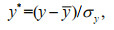 (1)
(1)where σy is the standard deviation of the monthly anomalies. The purpose of this data standardization technique was to eliminate the influence of the noise of the variables.
(2) The best-fit linear trend was then computed using linear regression analysis.
(3) The statistically significant trend was displayed as the one that exceeded the 95% confidence level, the correlation between CHL and the three environmental factors was calculated, and the relationships between CHL and the environmental factors were determined using multiple linear regression analysis.
3 RESULT 3.1 Monthly variation of CHL and environmental factorsTemporal analysis of the monthly averages CHL and the environment factors during 2003–2015 for our selected regions was performed. Although Regions 1 and Region 2 (or Regions 3–5) are located at the same latitudinal band, the variation of SST is different. As seen in Fig. 2, the SST of Region 1 shows an upward trend during January–March, a downward trend during March–September, and a further upward trend until December. In Region 2, SST increases during January–February, decreases during February– August, and increases during August–December. The SST of Region 3 decreases during January–February, increases during February–May, decreases slightly in June, increases during June–October, and then decreases until December. The pattern of SST variation in Region 4 is the opposite of that in Region 1. The patterns of change of SST in Region 5 is increase–decrease–increase–decrease. We found that the depth of the mixed layer was largely in the range of 20–100 m. The depth of the mixed layer in Regions 1 and 2 increases during January–February and decreases during February–June and increases until December. However, in Regions 3 and 4, it increases during January–August and then decreases during November–December. The changes of CHL and wind speed in each region are also different. The above analysis show that the seasonal patterns of CHL and environmental factors changes are not obvious.

|
| Fig.2 Variations of monthly averages (2003–2015) of SST, MLD, WS, and CHL in Regions 1-5 |
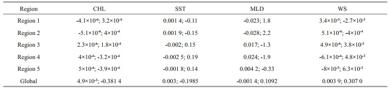
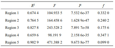
A 13-year time series of CHL was evaluated using linear regression analysis to assess the recent trend based on satellite observations from 2003–2015 (Fig. 3). In the five selected regions, noteworthy positive trends of CHL are apparent in Regions 3–5, whereas the trends in Regions 1 and 2 are negative, and the seasonal cycle of CHL is obvious (Fig. 3, Table 1). Regions 1 and 2 have increasing trends in SST and WS but decreasing trends in MLD. Increasing trends in MLD are observed in Regions 3–5 but the SST exhibits a trend of decrease. Regions 4 and 5 show a trend of decrease in WS, while Region 3 has a trend of increase. Higher ocean temperatures can produce a shallower mixed layer, allowing greater light availability in the mixed layer. A shallower upper MLD will probably lead to increased nutrient limitation and reduced nutrient exchange with deeper layers. We also calculated the slope and intercept of the trend line of the global CHL. Global CHL has an upward trend (Table 1), which is consistent with the results of Gregg et al. (2005) who reported an overall of 4.1% global increase in CHL for the same period.

|
| Fig.3 Time series of CHL, SST, MLD, and WS anomalies in Regions 1–5 The corresponding trend line is plotted as a dashed colored line. |
|
The correlations between CHL and the environmental factors were analyzed based on monthly observation datasets. Determining those environmental factors that are correlated with CHL is beneficial for understanding their interactions. The movement of the upper-level water of the selected regions primarily reflects a wind-driven circulation. The salinity and temperature provide the opportunity to calculate the density gradient. As the horizontal density gradient increases, the pycnocline and the nutriclines deepen, which influences the CHL concentration. Thus, the distribution of CHL is related to oceanic environmental factors (e.g., SST, MLD, and WS). The correlation between CHL and SST is negative in each selected region (Table 2). This might be because temperature influences CHL growth directly through its effect on the metabolic rate of organisms (Gregg et al., 2005; Feng et al., 2015). However, higher temperatures shorten the turnover times of plankton, produce a shallower MLD, and limit the nutrient supply. Thus, SST can regulate oceanic CHL indirectly (Gregg et al., 2005). The MLD is correlated positively with CHL, which indicates nutrient limitation (Lovenduski et al., 2008; Fay and Mckinley, 2017). Our results reveal that WS is an important factor in explaining the variance of CHL. The correlation coefficient between CHL and WS in Region 1 is positive, whereas it is negative in the other selected regions. The interesting correlation between CHL and WS is because some of the correlation is due to the direct influence of wind forcing on CHL, while some is due to the indirect influence of wind forcing on CHL. Upwelling or downwelling driven by the variability of winds affects the supply of nutrients, and therefore leads to an increase or decrease in CHL (Webster and Hutchinson, 1994; Wang et al., 2013), which illustrates the indirect effect of wind on CHL
Analysis of the environmental factors controlling CHL variability is an important scientific issue. Various methods including laboratory experiments and mathematical simulations are used to investigate the mechanisms via which such factors might influence CHL (Nezlin and Li, 2003). However, although it is known that CHL might be influenced by various independent variables (e.g., SST, MLD, and WS), exactly how these environmental factors might affect CHL is not yet fully understood. The correlation analysis described above found CHL correlated significantly with SST, MLD, and WS. In the following, the direct relationship between CHL and these environmental factors is explored using the multiple linear regression method based on observation datasets
The dependent variable (chl) can be denoted approximately as the linear function of independent variables (sst, mld, and ws). The full model incorporates by monthly environmental factors (sst, mld, and ws) effects as Eq.2:
 (2)
(2)where b0 is a constant, b1, b2, b3 are partial regression coefficients, (chl)t, (sst)t, (mld)t, and (ws)t are the monthly time series (t=1, 2, 3, ···, 156) of chl, sst, mld, and ws, the residual (err)t is the random error that excludes three entries independent variable influence to (chl)t. We first need to standardize each independent variable (sst, mld, and ws) and dependent variable (chl) for comparison with the effective intension of each independent variable (sst, mld, and ws) to chl. Modeling the impact of the environmental factors on CHL will allow us to simultaneously capture the linear effects of several variables. This model is used to explore the direct relationships between oceanic CHL and the environmental factors. Using the standardized data, the regression can be derived as follows:
 (3)
(3)and the corresponding regression coefficient is the standardization regression coefficient. If the absolute value of the standardization regression coefficient is large, the corresponding independent variable has large influence on the dependent variable (chl). The regression coefficients 


|
| Fig.4 Relational model between CHL and SST, MLD, and WS for Regions 1–5 The normal cumulative distribution of the residuals is shown in the right panel. |
Satellite-derived data of 2016 were used to validate our models and to determine whether the models respond well to the relationship between CHL and the environmental factors. The anomalies of CHL, SST, MLD, and WS were computed using Eq.1. The satellite-observed CHL and that calculated using our models in the selected regions are shown in Fig. 5. It can be seen that our models display satisfactory capability in depicting the relationship between CHL and the environmental factors in our selected regions. We tested the applicability of our models to the Northern Hemisphere, and the regression coefficients we chose were the averages of the regression coefficients for Regions 1 and 2. A similar methodology was adopted for the Southern Hemisphere. Overall, although the simulation results for the Northern (Southern) Hemisphere are less satisfactory than for the individual regions, they still capture the main change of CHL over time (Fig. 5f&g).

|
| Fig.5 Model validation based on satellite-derived data of 2016 Red lines with stars represent the observed CHL; blue lines with circles represent the results calculated by |
Many previous studies that focused on elucidating the impact of environmental factors on CHL considered only a single variable (i.e., SST, WS, or MLD) or only specific regions (George and Edwards, 1976; D'Sa and Korobkin, 2009; Kavak and Karadogan, 2012; Itoh et al., 2015; Ji et al., 2018). The referenced studies found that some physical processes (e.g., upwelling and mixing) drive the changes in oceanic CHL. The influence of physical processes on CHL is complex and the effects of environmental factors on CHL are interdependent. For example, as the regions we selected for this study are subject to wind forcing, their circulation strength will be adjusted accordingly. As the circulation strengthens, the horizontal density gradient will increase and both the pycnocline and the nutriclines will deepen. All these changes include variations in SST, MLD, and WS that work together to drive changes of CHL. Coupling between environmental factors complicates the problem. In our study, it is assumed that the effects of these environmental factors on CHL are independent. We selected five representative regions within the subtropical gyres, and developed models to describe the relationship between surface CHL and certain environmental factors. We analyzed the time series of anomalies in remote-sensed surface CHL concentration and their associated environmental factors. Regions 1 and 2 exhibited reasonably weak downward trends in CHL, whereas Regions 3–5 showed weak upward trends. Correlation analysis revealed significant relationships between CHL and the environmental factors. It was found that MLD (SST) was correlated positively (negatively) with CHL. Our regression coefficients showed that SST and MLD both had remarkable effect on CHL. Our model could be used to diagnose past change, understand present variability, and predict the future state of CHL changes based on environmental factors in the open ocean, which could help us develop greater understanding of the effect of these environmental factors on the distribution of oceanic CHL.
Although SST, MLD, and WS are the principal environmental factors controlling changes of CHL, in a realistic oceanic environment (Gregg et al., 2005; McQuatters-Gollop et al., 2008; Liu et al., 2012; Ji et al., 2018), ocean carbon absorption (Lovenduski et al., 2008; Fay and McKinley, 2017) could play an important role in changes of CHL. If ocean carbon absorption were considered, it could improve the accuracy of our models.
5 DATA AVALABILITY STATEMENTThe global CHL data is downloaded from (https://oceandata.sci.gsfc.nasa.gov/MODIS-Aqua/Mapped/Monthly/4km/chlor_a). SST data used in this study is available at (https://oceandata.sci.gsfc.nasa.gov/MODIS-Aqua/Mapped/Monthly/4km/sst). MLD is obtained from Argo data, the Argo data can be downloaded from (http://www.usgodae.org/argo/argo.html). Wind data can be downloaded from (http://www.remss.com/).
Behrenfeld M J, O'Malley R T, Siegel D A, McClain C R, Sarmiento J L, Feldman G C, Milligan A J, Falkowski P G, Letelier R M, Boss E S. 2006. Climate-driven trends in contemporary ocean productivity. Nature, 444(7120): 752-755.
DOI:10.1038/nature05317 |
Bentamy A, Grodsky S A, Carton J A, Croizé-Fillon D, Chapron B. 2012. Matching ASCAT and QuikSCAT winds. Journal of Geophysical Research: Oceans, 117(C2): C02011.
DOI:10.1029/2011JC007479 |
Chelton D B, Gaube P, Schlax M G, Early J J, Samelson R M. 2011a. The influence of nonlinear mesoscale eddies on near-surface oceanic chlorophyll. Science, 334(6054): 328-332.
DOI:10.1126/science.1208897 |
D'Sa E J, Korobkin M. 2009. Wind influence on chlorophyll variability along the Louisiana-Texas coast from satellite wind and ocean color data. In: Proceedings of SPIE7473, Remote Sensing of the Ocean, Sea Ice, and Large Water Regions 2009. SPIE, Berlin, Germany. 747305p, https://doi.org/10.1117/12.830537.
|
Fay A R, McKinley G A. 2017. Correlations of surface ocean pCO2 to satellite chlorophyll on monthly to interannual timescales. Global Biogeochemical Cycles, 31(3): 436-455.
DOI:10.1002/2016GB005563 |
Feng J F, Durant J M, Stige L C, Hessen D O, Hjermann D Ø, Zhu L, Llope M, Stenseth N C. 2015. Contrasting correlation patterns between environmental factors and chlorophyll levels in the global ocean. Global Biogeochemical Cycles, 29(12): 2095-2107.
DOI:10.1002/2015GB005216 |
George D G, Edwards R W. 1976. The Effect of wind on the distribution of chlorophyll a and crustacean plankton in a shallow eutrophic reservoir. Journal of Applied Ecology, 13(3): 667-690.
DOI:10.2307/2402246 |
Gregg W W, Casey N W, McClain C R. 2005. Recent trends in global ocean chlorophyll. Geophysical Research Letters, 32(3): L03606.
DOI:10.1029/2004GL021808 |
Huang R X, Russell S. 1994. Ventilation of the subtropical north pacific. Journal of Physical Oceanography, 24(12): 2589-2605.
DOI:10.1175/1520-0485(1994)024<2589:votsnp>2.0.co;2 |
Itoh S, Yasuda I, Saito H, Tsuda A, Komatsu K. 2015. Mixed layer depth and chlorophyll a: Profiling float observations in the Kuroshio-Oyashio extension region. Journal of Marine Systems, 151: 1-14.
DOI:10.1016/j.jmarsys.2015.06.004 |
Ji C X, Zhang Y Z, Cheng Q M, Tsou J Y, Jiang T C, Liang X S. 2018. Evaluating the impact of sea surface temperature(SST) on spatial distribution of chlorophyll-a concentration in the East China Sea. International Journal of Applied Earth Observation and Geoinformation, 68: 252-261.
DOI:10.1016/j.jag.2018.01.020 |
Kavak M T, Karadogan S. 2012. The relationship between sea surface temperature and chlorophyll concentration of phytoplanktons in the Black Sea using remote sensing techniques. Journal of Environmental Biology, 33(2 Suppl.): 493-498.
|
Killworth P D, Cipollini P, Uz B M, Blundell J R. 2004. Physical and biological mechanisms for planetary waves observed in satellite-derived chlorophyll. Journal of Geophysical Research: Oceans, 109(C7): C07002.
DOI:10.1029/2003JC001768 |
Liu F F, Chen C Q, Zhan H G. 2012. Decadal variability of chlorophyll a in the South China Sea: a possible mechanism. Chinese Journal of Oceanology and Limnology, 30(6): 1054-1062.
DOI:10.1007/s00343-012-1282-9 |
Longhurst A. 1993. Seasonal cooling and blooming in tropical oceans. Deep Sea Research Part Ⅰ: Oceanographic Research Papers, 40(11-12): 2145-2165.
DOI:10.1016/0967-0637(93)90095-K |
Lovenduski N S, Gruber N, Doney S C. 2008. Toward a mechanistic understanding of the decadal trends in the Southern Ocean carbon sink. Global Biogeochemical Cycles, 22(3): GB3016.
DOI:10.1029/2007GB003139 |
McClain C R, Signorini S R, Christian J R. 2004. Subtropical gyre variability observed by ocean-color satellites. Deep Sea Research Part Ⅱ: Topical Studies in Oceanography, 51(1-3): 281-301.
DOI:10.1016/j.dsr2.2003.08.002 |
McQuatters-Gollop A, Mee L D, Raitsos D E, Shapiro G I. 2008. Non-linearities, regime shifts and recovery: The recent influence of climate on Black Sea chlorophyll. Journal of Marine Systems, 74(1-2): 649-658.
DOI:10.1016/j.jmarsys.2008.06.002 |
Nezlin N P, Li B L. 2003. Time-series analysis of remotesensed chlorophyll and environmental factors in the Santa Monica-San Pedro Basin off Southern California. Journal of Marine Systems, 39(3-4): 185-202.
DOI:10.1016/S0924-7963(03)00030-7 |
Qiu F W, Fang W D, Fang G H. 2011. Seasonal-to-interannual variability of chlorophyll in central western South China Sea extracted from SeaWiFS. Chinese Journal of Oceanology and Limnology, 29(1): 18-25.
DOI:10.1007/s00343-011-9931-y |
Raymont J E G. 1980. Plankton and Productivity in the Oceans. Phytoplankton, vol. 1.2nd edn. Pergamon, Oxford. 489p.
|
Uz B M, Yoder J A. 2004. High frequency and mesoscale variability in SeaWiFS chlorophyll imagery and its relation to other remotely sensed oceanographic variables. Deep Sea Research Part Ⅱ: opical Studies in Oceanography, 51(10-11): 1001-1017.
DOI:10.1016/j.dsr2.2004.03.003 |
Wang D K, Wang H, Li M, Liu M M, Wu X Y. 2013. Role of Ekman transport versus Ekman pumping in driving summer upwelling in the South China Sea. Journal of Ocean University of China, 12(3): 355-365.
DOI:10.1007/s11802-013-1904-7 |
Webster I T, Hutchinson P A. 1994. Effect of wind on the distribution of phytoplankton cells in lakes revisited. Limnology and Oceanography, 39(2): 365-373.
DOI:10.4319/lo.1994.39.2.0365 |
Wentz F J. 1997. A well-calibrated ocean algorithm for special sensor microwave/imager. Journal of Geophysical Research: Oceans, 102(C4): 8703-8718.
DOI:10.1029/96JC01751 |