 2021, Vol. 39
Institute of Oceanology, Chinese Academy of Sciences
Article Information
- CUI Chaoran, ZHANG Rong-Hua, WEI Yanzhou, WANG Hongna
- Mesoscale wind stress-SST coupling induced feedback to the ocean in the western coast of South America
- Journal of Oceanology and Limnology, 39(3): 785-799
- http://dx.doi.org/10.1007/s00343-020-0182-7
Article History
- Received May. 2, 2020
- accepted in principle Jun. 5, 2020
- accepted for publication Jun. 16, 2020


2 University of Chinese Academy of Sciences, Beijing 100049, China;
3 Qingdao National Laboratory for Marine Science and Technology, Qingdao 266000, China;
4 Center for Excellence in Quaternary Science and Global Change, Chinese Academy of Sciences, Xi'an 710061, China;
5 State Key Laboratory of Satellite Ocean Environment Dynamics, Second Institute of Oceanography, Ministry of Natural Resources, Hangzhou 310012, China
Mesoscale air-sea coupling is a salient process that is prominent in the regions with energetic eddies and fronts. It is often characterized by a positive correlation between sea surface temperature (SST) perturbations (SST▽meso) and wind stress perturbations (WSmeso) at a typical length of 10-100 km. The influence of mesoscale SST perturbations on the surface wind stress was previously observed by Sweet et al. (1981), who found that the magnitude of cross-front wind stress increased when the wind passed from cold to warm water in the Gulf Stream. Mesoscale air-sea coupling is also characterized by a linear correlation between wind stress divergence (curl) perturbations Div(WS)meso (Curl(WS)meso) and downwind (crosswind) SST gradient perturbations▽downSSTmeso (▽crossSSTmeso) (Chelton et al., 2004, 2007). These relationships have been verified by observations and model simulations (Shaw et al., 1999; Chelton et al., 2001; Bourras, 2004; O'Neill et al., 2005; Small et al., 2008; Castelao, 2012; O'Neill, 2012).
The mesoscale air-sea coupling can be well described by two mechanisms (Chelton et al., 2007; Small et al., 2008; Chelton and Xie, 2010; Desbiolles et al., 2018; Gao et al., 2019). The first is related to downwind momentum transport. SSTmeso can modify the turbulent mixing within the marine atmospheric boundary layer, and then the downward momentum transport is changed and generates advective acceleration of near-surface wind from cool to warm SST and deceleration of near-surface wind from warm to cool SST. The second mechanism is related to the sea level pressure adjustment. Observations show that WSmeso in the upstream (downstream) of warm SSTmeso is accelerated (decelerated) due to sea level pressure anomalies above SSTmeso.
A strong eastern boundary upwelling exists in the western coast of South America (Albert et al., 2010; Oerder et al., 2015). The strong wind-forced upwelling supplies rich nutrients in this region, producing a productive ecosystem that provides much of the world's fish catch (Chavez et al., 2008). Furthermore, this region plays an important role in the global climate because of its effect on the El Niño-Southern Oscillation (Ma et al., 1996). Model simulations have been a powerful approach to understand and predict the upwelling system in this region and its climate effects. However, there is a consistent warm SST bias in most of climate model simulations in this region (Zuidema et al., 2016; Zhu and Zhang, 2018, 2019; Zhang et al., 2020). This bias in the tropical ocean may be affected by cloud liquid water path and stratus cloud coverage represented in atmospheric models, which leads to an excessive amount of solar radiation that is received at the sea surface (Ma et al, 1996; Davey et al., 2002; Meehl et al., 2005; Huang et al., 2007; Hu et al., 2011).
Note that strong mesoscale air-sea coupling occurs in the western coast of South America because of intense mesoscale eddy activities. Previous studies have showed that mesoscale wind stress-SST coupling can have important feedback to the atmosphere and ocean (Zhang and Busalacchi, 2008; Hogg et al., 2009; Frenger et al., 2013; Zhang et al., 2014; Zhang, 2014; Ma et al., 2016; Wei et al., 2017). Piazza et al. (2016) showed the mesoscale coupling had an upscale effect on the tropospheric wind and storm in the Gulf Stream. Particularly, as the change in wind stress curl induced by mesoscale coupling can impact the Ekman pumping, the mesoscale wind stress-SST coupling can exert an important feedback to the upwelling system, which may affect SST in this region (Bakun, 1990; Jin et al., 2009; Albert et al., 2010; Gaube et al., 2015; Seo et al., 2016). Indeed, Penven et al. (2005) showed that the warm SST bias in climate models might be a consequence of their incapacity to accurately resolve the nearshore upwelling and eddy activities. Therefore, it is necessary to study the feedback induced by the mesoscale air-sea coupling to the ocean in this region, which may potentially reduce the warm SST bias in many climate models.
Using a high resolution Weather Research and Forecasting (WRF) and Nucleus for European Modeling of the Ocean (NEMO) model, Oerder et al. (2016) showed that WSmeso response to SSTmeso in the western coast of South America was mainly attributed to turbulent momentum transport in the atmospheric boundary layer, with the coupling coeffcient between WSmeso and SSTmeso in austral winter being larger than that in austral summer. They also showed that the intensity of mesoscale eddy activities was reduced if the effect of surface ocean current on the wind stress was taken into account in the model (Oerder et al., 2018). However, there are few studies focusing on the feedback induced by the mesoscale wind stress-SST coupling in this region. Therefore, we aim to study the feedback induced by mesoscale wind stress-SST coupling to the ocean in the western coast of South America. As ocean-only models and coarse-resolution climate models cannot adequately represent the characteristics of mesoscale wind stress-SST coupling (Bryan et al., 2010), we explore an empirical approach to parameterize WSmeso from SSTmeso gradients, and incorporate it in the ocean model to examine the effect on ocean simulation.
The paper is organized as follows: Section 2 describes the empirical wind stress perturbation model, the ocean model and experimental configuration. Section 3 reports the feedback induced by the mesoscale wind stress-SST coupling to the ocean simulation in the western coast of South America. Section 4 examines the processes by which the mesoscale coupling impacts the SST, and Section 5 presents a summary.
2 METHODOLOGY 2.1 Observed dataThe satellite data are used to quantify the mesoscale SST-wind stress coupling relationship in this study. The daily wind stress data are derived from Quick Scatterometer (Quik-SCAT, Version 4) which are launched from July 1999 to November 2009. The AMSR-E SST data are available from June 2002 to September 2011. For this study, we use the daily data with spatial resolution of 0.25° for period from June 2002 to November 2009. All of the data are obtained from the Asia-Pacific Data-Research Center (APDRC) of the University of Hawaii.
2.2 An empirical wind stress perturbation modelA locally weighted regression (LOESS) method (Cleveland and Devlin, 1988) is used to extract the SSTmeso and WSmeso in the western coast of South America. The mesoscale perturbations of a field φ (SST or wind stress magnitude) are defined as 

 (1)
(1)in which m=d/dmax, d is the distance between target point and a surrounding point, dmax is the maximum distance between target point and each point in the spatial filter window.
The regression function is
 (2)
(2)in which x and y denote the coordinates relative to the target point. α1 equals
The magnitude of the derived perturbations depends on the half-span parameter used in the LOESS method. In order to extract the mesoscale perturbations effciently in the western coast of South America, the half-span parameter is taken as 10° according to previous results (Cui et al., 2020).
To determine WSmeso effectively for use in the ocean model, the Tikhonov regularization method is used to calculate WSmeso from the Curl(WSmeso) and Div(WSmeso), which are approximated from modeled ▽downSSTmeso and ▽crossSSTmeso using their empirical relationships obtained from satellite observations. Details of the method can be found in Wei et al.(2017, 2018) and Cui et al. (2020).
2.3 Ocean modelThe ocean model used in this study is the Regional Ocean Modeling System (ROMS) version 3.4. ROMS is a three-dimensional, free surface and terrain-following numerical model. It solves hydrostatic and primitive equations using a short time step for the surface elevation and barotropic momentum equations, and a longer time step for 3D temperature, salinity and baroclinic momentum equations (Song and Haidvogel, 1994; Shchepetkin and McWilliams, 2005). ROMS provides several schemes for mixing parameterizations. This study takes the harmonic mixing scheme for horizontal mixing and the Mellor/Yamada Level-2.5 closure parameterization scheme for vertical mixing (Wajsowicz, 1993). Horizontal tracer and momentum advection are treated using a third-order upstream discretization scheme. The vertical advection is evaluated using the fourth-order centered discretization scheme. Details of the ROMS computational algorithms are described by Shchepetkin and McWilliams (2005).
To resolve the mesoscale phenomenon in the region and its interactions with basin-scale ocean circulation in the tropical Pacific, we configured a nested modeling system using ROMS with two different domains at high and low spatial resolutions, respectively. The larger domain covers the whole tropical Pacific from 35°S to 35°N and from 100°E to 70°W with a horizontal grid resolution of 1/2°×1/2°cosΦ (Φ is latitude). The small inner domain extends from 30°S to 0°N and from 95°W to 70°W in the western coast of South America; the horizontal grid resolution of inner domain is 1/8°×1/8°cosΦ (Φ is latitude). In the vertical direction, there are 40 levels (s-coordinate) of the inner domain with higher vertical resolution near the surface and bottom (Song and Haidvogel, 1994; Haidvogel et al., 2008). The bottom topographies in both domains are obtained from the Global 2-min Gridded Topographic Data ETOPO2. The ETOPO2 data set was generated from a digital database of seafloor and land elevations, which includes the satellite altimeter data, shipboard echo-sounding measurements, and data from global digital elevation model. Note that the eastern boundary is closed and other three (northern, southern, and western) boundaries are open for both the domains. The depth ranges from 75 m to 5 000 m. To make long-term integrations more stable, radiation-nudging boundary conditions are used with a 360-day time scale for outflow and 3-day time scale for inflow. The time steps are 30 s for the 2-D barotropic equations, and 300 s for the 3-D baroclinic equations.
The Quik-SCAT monthly mean surface wind fields during 2003-2008 are used to force the ocean model. Air-sea fluxes are calculated by the bulk formulae from atmosphere parameters (the National Center for Environmental Prediction (NCEP) reanalysis product during 1985-2015, including monthly mean relative humidity, solar shortwave radiation, longwave radiation, precipitation, surface air pressure, and surface air temperature). The initial and boundary conditions for the larger-domain model are specified from the World Ocean Atlas 2009 (WOA 2009), which is a set of objectively analyzed climatological hydrographic data for ocean parameters from 0 m at the surface to 5 500 m at the bottom. The larger-domain model is run for 30 years and its monthly mean outputs provide initial and boundary conditions for the inner-domain model. The inner-domain model is also run for 30 years to get a quasi-equilibrium state of 3-D velocity, temperature, and salinity, as well as the 2-D sea surface elevation.
2.4 Sensitivity experimentTo assess the feedback due to mesoscale coupling to the ocean in the western coast of South America, four experiments are designed. The first experiment is a control one with model settings described above. The second one is the mesoscale coupling experiment, in which the effect of mesoscale coupling is included by calculating the WSmeso from its empirical model in ROMS. The WSmeso is derived from Curl(WSmeso) and Div(WSmeso) which are approximated from modeled ▽downSSTmeso and ▽crossSSTmeso at each time step. Then, the mesoscale wind speed perturbation (WSPDmeso) is obtained from the WSmeso and added to the monthly mean wind speed, which modifies the surface wind stress and heat flux based on the bulk formula.
Other two experiments are designed to investigate the separate feedback of mesoscale coupling to the ocean associated with heat flux and momentum flux, respectively. They are referred to as the HF-feedback experiment (only the influence of WSPDmeso on surface heat flux (HF) is considered) and the MFfeedback experiment (only the influence of WSmeso on surface wind stress (momentum flux; MF) is considered), respectively.
These four experiments all start from the beginning of the 31st year of model simulation, and are run for 10 years to investigate the effect of mesoscale air-sea coupling on long-term mean ocean simulations.
3 FEEDBACK DUE TO MESOSCALE COUPLING TO THE OCEAN 3.1 Simulated mesoscale SST and wind stress perturbationsFigure 1 shows mesoscale perturbation fields of AMSR-E SST and Quik-SCAT wind stress magnitude in April 2007. The field of WSmeso magnitude is highly consistent with that of SSTmeso, and the wind slows down over cooler waters and speeds up over warmer waters. It is evident that the LOESS method can isolate the mesoscale signals effciently from the large-scale background field. Figure 2a-b shows the simulated long-term mean SSTmeso and WSmeso in the western coast of South America, respectively. It is clearly seen that the characteristic SSTmeso and WSmeso features in observations can be well captured. The regions with large SSTmeso are in the nearshore area of Peru Sea and Chile Sea both in the observations and simulated outputs. The reconstructed WSmeso is closely related to that of simulated SSTmeso (Fig. 2a-b). As shown in Fig. 3, the coupling coeffcient between SSTmeso and WSmeso in simulation (0.007 6 ℃/(N/m2)) is nearly equal to that in observations (0.006 5 ℃/(N/m2)). These results indicate that WSmeso can be well represented from the SSTmeso using the empirical model calculated by the Tikhonov's regularization method.

|
| Fig.1 Spatially high pass filtered AMSR-E SST (a) and Quik-SCAT wind stress (b) magnitude in April 2007 |

|
| Fig.2 The simulated mesoscale SST (a) and wind stress (b) magnitude perturbations which are averaged from the 31st to the 40th year in ROMS |

|
| Fig.3 The coupling coeffcients between wind stress and SST perturbations in observations (Quik-SCAT wind stress and AMSR-E SST data during 2003-2008) (a) and ROMS model simulation (b) The black dots and vertical bars indicate the medians and interquartile ranges in each bin. |
To diagnose the feedback induced by mesoscale coupling on SST, the mesoscale coupling experiment (described in Section 2.4) is conducted. Figure 4 shows the mean SST difference between the two experiments. Obviously, SST is reduced in the offshore areas of the Peru and Chile Sea in the mesoscale coupling experiment. The reduced maximum values of SST can reach 0.5 ℃ in the Peru Sea and 0.7 ℃ in the Chile Sea. It is worth noting that there is positive SST difference in nearshore sea area.

|
| Fig.4 The mean SST difference between the mesoscale coupling experiment and control experiment |
The physical processes that lead to the SST difference are examined by the mixed layer (ML) heat budget analysis. The mixed layer depth (MLD) is defined as the depth at which the density increases by 0.125 kg/m3 from the sea surface (Chelton et al., 2007). The vertically averaged ML heat budget equation is derived from the conservation of temperature equation:
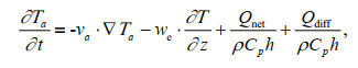 (3)
(3)where h is MLD; T and v are temperature and horizontal currents; subscript a represents quantities that are vertically averaged between the surface and h; ρ is the density of seawater; Cp is heat capacity of sea water; Qnet is the difference between downward surface heat flux and shortwave radiation transmitted through the bottom of ML Qpen; we is entrainment velocity across the bottom of ML, calculated by:
 (4)
(4)in which w-h is the vertical velocity at the bottom of the mixed layer. Qpen is calculated by:
 (5)
(5)in which Qshort is the shortwave radiation, and Qdiff is the diffusive heat flux at the bottom of ML:
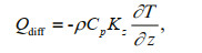 (6)
(6)in which Kz is the function of Richardson number. Details of the computation of heat budget in the ML were described by Huang et al. (2010).
The left-hand side of Eq.3 is the ML temperature tendency, which is determined by terms on the right-hand side. The first term on the right-hand side is the horizontal advection caused by depth-averaged current. The second term is the vertical entrainment. The third and fourth terms are the adjusted surface heat flux and vertical heat diffusion at the bottom of ML, respectively. Figure 5 shows the differences in each heat budget term between the mesoscale coupling experiment and control experiment. The difference in temperature tendency is not coherent and thus is not shown. The horizontal advection and surface heat flux are the main terms that explain the difference in SST (Fig. 5a-b). The horizontal advection tends to decrease the SST in the offshore area and increase the SST in the nearshore area, which is consistent with SST differences induced by the feedback of mesoscale coupling. The surface heat flux has an opposite effect to the SST difference. The contributions of vertical entrainment and vertical heat diffusion terms are relatively small. They tend to damp the positive SST difference in the nearshore of Peru Sea (Fig. 5c-d).

|
| Fig.5 The differences in surface heat flux (a), horizontal advection (b), vertical entertainment (c), and vertical diffusion (d) in mixed layer heat budget equation between the mesoscale coupling experiment and control experiment |
To further analyze the contribution of surface heat flux term to SST, the differences in latent heat flux, upward longwave radiation and sensible heat flux between the mesoscale coupling experiment and control experiment are presented in Fig. 6. The latent heat flux is affected by wind speed and the temperature difference between the atmosphere and ocean surface based on the bulk flux formulae. As shown in Fig. 6a, the difference in latent heat flux is closely related to that in SST (Fig. 4), which means the effect due to the SST difference on latent heat flux is more important than wind speed in this region. The changed upward latent heat flux in turn acts to damp the SST difference. The similar results are found in upward longwave radiation and sensible heat flux (Fig. 6b-c). It can be concluded that surface heat flux mainly acts to damp the SST difference in the western coast of South America; a similar case can be seen in the Kuroshio extension (Wei et al., 2017).

|
| Fig.6 The differences in latent heat flux (a), upward longwave radiation (b), and sensible heat flux (c) between the mesoscale coupling experiment and control experiment |
Figure 7 shows the long-term mean horizontal current in the control experiment and their differences between the mesoscale coupling experiment and control experiment. The results are vertically averaged in the mixed layer. Because of the strong westward wind, there is strong zonal offshore current in the western coast of South America (Fig. 7a). The meridional current is northward in the nearshore area (Fig. 7c). The mesoscale coupling exerts a profound feedback to horizontal current. Consistent with the negative WSmeso induced by negative SSTmeso in the nearshore sea, the meridional and zonal current velocities are both weakened in these regions (Fig. 7b & d). As the difference in SST is mainly determined by horizontal advection, the weakened horizontal currents in the nearshore sea is responsible for the positive SST difference.

|
| Fig.7 The long-term mean zonal (a) and meridional (c) current components in the control experiment; the differences in zonal (b) and meridional (d) current components between the mesoscale coupling experiment and control experiment |
The long-term mean vertical current component in the control experiment and its difference between the mesoscale coupling experiment and control experiment are shown in Fig. 8. The results are vertically averaged in the mixed layer. The vertical flow is upward in the nearshore sea area and downward in the offshore sea area (Fig. 8a). When the feedback induced by mesoscale coupling to the ocean is incorporated into the model simulation, it is obvious that upward vertical velocity is strengthened in the nearshore sea (Fig. 8b). Previous studies have found that Ekman pumping can be modulated by the curl of WSmeso especially in the region with intense mesoscale eddy activities (Gaube et al., 2015; Seo et al., 2016; Seo, 2017). To examine whether the difference in vertical velocity is related to the Ekman pumping induced by curl of WSmeso, the difference in wind stress curl between the mesoscale coupling experiment and control experiment is given in Fig. 8c. It shows that the difference in vertical current is consistent with that in wind stress curl, indicating the difference in vertical velocity is mainly attributed to the difference in Ekman pumping induced by curl of WSmeso. In summary, the ocean current velocity is substantially affected by mesoscale coupling in the western coast of South America. The strengthened Ekman pumping can bring subsurface cold water to the sea surface and lead to the cooling of SST.

|
| Fig.8 The long-term mean vertical current component in the control experiment (a); the difference in vertical current component between the mesoscale coupling experiment and control experiment (b); the difference in wind stress curl between the mesoscale coupling experiment and control experiment (c) |
The feedback effect of mesoscale wind stress-SST coupling on the ocean displays seasonal variation. Figure 9 shows the differences in SST between the mesoscale coupling experiment and control experiment in four seasons. The difference in SST is relatively large in austral summer (February-April) and small in austral winter (August-October). By analyzing heat budget terms in the ML, it is found that the cooling tendency in SST is attributed to horizontal advection, vertical entrainment, and vertical heat diffusion both in austral summer and winter. The contributions of horizontal advection, vertical entrainment, and vertical heat diffusion terms in austral summer are larger than those in winter. The vertical velocity differences induced by feedback of the mesoscale coupling in four seasons are given in Fig. 10. As discussed above, the difference in vertical velocity is mainly attributed to Ekman pumping induced by curl of WSmeso. Thus, the difference in vertical velocity is consistent with that in WSmeso curl in all seasons (not shown). Figure 10 also shows the upwelling in the offshore area of Peru Sea in austral winter is weaker than that in summer. The weakened upwelling reduces the transport of subsurface cold water to sea surface, which can be one factor inducing the less cooled SST in austral winter.

|
| Fig.9 The differences in SST in austral spring (November-January) (a), austral summer (February-April) (b), austral autumn (May-July) (c), and austral winter (August-October) (d) between the mesoscale coupling experiment and control experiment |

|
| Fig.10 The differences in vertical current in austral spring (November–January) (a), austral summer (February–April) (b), austral autumn (May–July) (c), and austral winter (August–October) (d) between the mesoscale coupling experiment and control experiment |
We have shown that the incorporation of mesoscale coupling into the model can lead to SST difference in the western coast of South America. The difference in SST can be determined by momentum flux (MF) and heat flux (HF), since mesoscale wind forcing can alter the surface wind stress and surface heat flux directly. To examine the way by which the mesoscale coupling impacts the SST, the HF-feedback experiment (only the influence of WSmeso on surface heat flux is considered) and MF-feedback experiment (only the influence of WSmeso on surface wind stress is considered) are conducted (Table. 1), and results are presented in this section. Details of two experiments are described in Section 2.4.
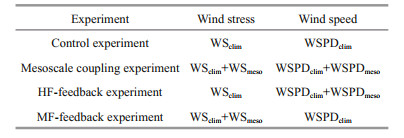
Figure 11 shows the differences in SST between the two sensitivity experiments and control experiment. In the MF-feedback experiment, the reduced maximum values of SST are about 0.5 ℃ both in Peru Sea and Chile Sea (Fig. 11a). In the HF-feedback experiment, the regions with large difference in SST are mainly in the Chile Sea with maximum reduced value being about 0.3 ℃ (Fig. 11b). The SST difference between the mesoscale coupling experiment and control experiment is generally a sum of the SST differences between the two sensitivity experiments and control experiment. Heat budget analysis also indicates that the SST difference is mainly determined by horizontal advection and surface heat flux in both the sensitivity experiments.

|
| Fig.11 The differences in SST between the MF-feedback experiment and control experiment (a) and HF-feedback experiment and control experiment (b) |
In addition, the differences in sea surface heat flux between the two sensitivity experiments and control experiment are shown in Fig. 12. The latent heat flux is affected by wind speed and temperature difference between the atmosphere and ocean surface. As wind speed is not allowed to be affected by wind speed perturbations due to SSTmeso in MF-feedback experiment, the difference in latent heat flux is well related to that in mean SST (Figs. 11a & 12a). The similar results are found in the upward longwave radiation and sensible heat flux (Fig. 12b & c). In HF-feedback experiment, the difference in latent heat flux (Fig. 12d) is mainly determined by wind speed perturbations induced by SSTmeso, whereas the differences in upward longwave radiation and sensible heat flux are mainly determined by mean SST difference (Fig. 12e & f).

|
| Fig.12 The differences in latent heat flux (a), upward longwave radiation (b), and sensible heat flux (c) between the MFfeedback experiment and control experiment; the difference in latent heat flux (d), upward longwave radiation (e), and sensible heat flux (f) between the HF-feedback experiment and control experiment |
In this work, the feedback effect induced by the mesoscale wind stress-SST coupling on the ocean in the western coast of South America is investigated by numerical simulations. Firstly, according to the coupling relationships between Div(WSmeso) (Curl(WSmeso)) and ▽downSSTmeso (▽crossSSTmeso) derived from the satellite data, Div(WSmeso) and Curl(WSmeso) are obtained from SST gradient perturbations simulated from the ROMS. Then, WSmeso is derived from Div(WSmeso) and Curl(WSmeso) by the Tikhonov regularization method and incorporated into the ROMS to represent its effect on the ocean. After including the feedback of mesoscale wind stress-SST coupling in the ROMS, SST can be reduced in the offshore area of the Peru and Chile Sea. The maximum reduced values can reach 0.5 ℃ in the Peru Sea and 0.7 ℃ in the Chile Sea.
Based on the mixed layer heat budget analysis, we find that horizontal advection and surface heat flux are the main terms that explain the difference in SST between the mesoscale coupling experiment and control experiment. The horizontal advection term has a positive contribution to the SST difference with the cooling in offshore area and slightly warming in the nearshore area. However, the surface heat flux has a negative effect on the SST difference. Vertical entrainment and vertical heat diffusion act to damp the SST warming in the nearshore of Peru Sea. The feedback due to mesoscale coupling to the ocean also leads to strengthened vertical velocity in the nearshore sea area, which is mainly attributed to the Ekman pumping induced by curl of WSmeso.
The cooling SST induced by mesoscale wind stress-SST coupling is relatively large in austral summer (February-April) and small in austral winter (August-October). By analyzing the heat budget terms in the ML, it is found that the SST cooling is primarily contributed by the horizontal advection term both in austral summer and winter. Meanwhile, there is weaker upwelling in the offshore area of Peru Sea in austral winter than in austral summer. The weakened upwelling reduces the transport of subsurface cold water to sea surface; this can be one reason why SST is less cooled in austral winter.
The way by which the mesoscale coupling affects the SST in the western coast of South America is examined further by two sensitivity experiments. In the MF-feedback experiment (only the influence of WSmeso on surface wind stress is considered), the reduced values of SST are about 0.5 ℃ both in the Peru Sea and Chile Sea. In the HF-feedback experiment (only the influence of WSmeso on surface heat flux is considered), the regions with large SST difference (>0.3 ℃) are mainly in the Chile Sea. By analyzing the heat budget terms in ML, horizontal advection and surface heat flux are also the main terms that explain the SST differences between the two sensitivity experiments and control experiment.
Thus, the mesoscale wind stress-SST coupling can have important feedback effect on the ocean in the western coast of South America. The feedback induced by mesoscale wind stress-SST coupling can reduce SST by a maximum of 0.5 ℃ in the Peru Sea and 0.7 ℃ in the Chile Sea, which may potentially reduce the warm SST bias in current climate models and improve the ocean simulations in the western coast of South America.
Although the computational application in this study is located in the western coast of South America, the empirical model constructed by the Tikhonov's regularization method can be applicable to any regions and useful for the study of mesoscale coupling. As it is difficult to well simulate the atmospheric wind response to SSTmeso in the climate models with simulated coupling coefficient between WSmeso and SSTmeso being smaller than observations (Bryan et al., 2010), the empirical model can be used to represent WSmeso in response to SSTmeso. This method can help shed light on better understanding of the physical processes that are involved in the mesoscale SSTwind coupling and improve the model simulations.
6 DATA AVAILABILITY STATEMENTAll the satellite data are obtained from the AsiaPacific Data-Research Center (APDRC) of the University of Hawaii, which is available at http://apdrc.soest.hawaii.edu/las/v6/dataset?catitem=1. The model data and computer codes used in this paper are available from the authors (e-mail: rzhang@qdio.ac.cn).
7 ACKNOWLEDGMENTThe authors wish to thank the anonymous reviewers for their comments that helped to improve the original manuscript.
Albert A, Echevin V, Lévy M, Aumont O. 2010. Impact of nearshore wind stress curl on coastal circulation and primary productivity in the Peru upwelling system. J. Geophys. Res.: Oceans, 115(C12): C12033.
DOI:10.1029/2010JC006569 |
Bakun A. 1990. Global climate change and intensification of coastal ocean upwelling. Science, 247(4939): 198-201.
DOI:10.1126/science.247.4939.198 |
Bourras D, Reverdin G, Giordani H, Caniaux G. 2004. Response of the atmospheric boundary layer to a mesoscale oceanic eddy in the northeast Atlantic. J. Geophys. Res.: Atmos., 109(D18): D18114.
DOI:10.1029/2004JD004799 |
Bryan F O, Tomas R, Dennis J M, Chelton D B, Loeb N G, McClean J L. 2010. frontal scale air-sea interaction in high-resolution coupled climate models. J. Climate, 23(23): 6 277-6 291.
DOI:10.1175/2010JCLI3665.1 |
Castelao R M. 2012. Sea surface temperature and wind stress curl variability near a cape. J. Phys. Oceanogr., 42(11): 2 073-2 087.
DOI:10.1175/JPO-D-11-0224.1 |
Chavez F P, Bertrand A, Guevara-Carrasco R, Soler P, Csirke J. 2008. The northern Humboldt Current system: brief history, present status and a view towards the future. Prog. Oceanogr., 79(2-4): 95-105.
DOI:10.1016/j.pocean.2008.10.012 |
Chelton D B, Esbensen S K, Schlax M G, Thum N, Freilich M H, Wentz F J, Gentemann C L, McPhaden M J, Schopf P S. 2001. Observations of coupling between surface wind stress and sea surface temperature in the eastern tropical Pacific. J. Climate, 14(7): 1 479-1 498.
DOI:10.1175/1520-0442(2001)014<1479:OOCBSW>2.0.CO;2 |
Chelton D B, Schlax M G, Freilich M H, Milliff R F. 2004. Satellite measurements reveal persistent small-scale features in ocean winds. Science, 303(5660): 978-983.
DOI:10.1126/science.1091901 |
Chelton D B, Schlax M G, Samelson R M. 2007. Summertime coupling between sea surface temperature and wind stress in the California current system. J. Phys. Oceanogr., 37(3): 495-517.
DOI:10.1175/JPO3025.1 |
Chelton D B, Xie S P. 2010. Coupled ocean-atmosphere interaction at oceanic mesoscales. Oceanography, 23(4): 52-69.
DOI:10.5670/oceanog.2010.05 |
Cleveland W S, Devlin S J. 1988. Locally weighted regression: an approach to regression analysis by local fitting. J. Am. Stat. Assoc., 83(403): 596-610.
DOI:10.2307/2289282 |
Cui C R, Zhang R H, Wang H N, Wei Y Z. 2020. Representing surface wind stress response to mesoscale SST perturbations in western coast of South America using Tikhonov regularization method. J. Oceanol. Limnol., 38(3): 679-694.
DOI:10.1007/s00343-019-9042-8 |
Davey M, Huddleston M, Sperber K, Braconnot P, Bryan F, Chen D, Colman R, Cooper C, Cubasch U, Delecluse P, DeWitt D, Fairhead L, Flato G, Gordon C, Hogan T, Ji M, Kimoto M, Kitoh A, Knutson T, Latif M, Le Treut H, Li T, Manabe S, Mechoso C, Meehl G, Power S, Roeckner E, Terray L, Vintzileos A, Voss R, Wang B, Washington W, Yoshikawa I, Yu J, Yukimoto S, Zebiak S. 2002. STOIC: a study of coupled model climatology and variability in tropical ocean regions. Climate Dyn., 18(5): 403-420.
DOI:10.1007/s00382-001-0188-6 |
Desbiolles F, Blamey R, Illig S, James R, Barimalala R, Renault L, Reason C. 2018. Upscaling impact of wind/sea surface temperature mesoscale interactions on southern Africa austral summer climate. Int. J. Climatol., 38(12): 4 651-4 660.
DOI:10.1002/joc.5726 |
Frenger I, Gruber N, Knutti R, Münnich M. 2013. Imprint of Southern Ocean eddies on winds, clouds and rainfall. Nat. Geosci., 6(8): 608-612.
DOI:10.1038/ngeo1863 |
Gao J X, Zhang R H, Wang H N. 2019. Mesoscale SST perturbation-induced impacts on climatological precipitation in the Kuroshio-Oyashio extension region, as revealed by the WRF simulations. J. Oceanol. Limnol., 37(2): 385-397.
DOI:10.1007/s00343-019-8065-5 |
Gaube P, Chelton D B, Samelson R M, Schlax M G, O'Neill L W. 2015. Satellite observations of mesoscale eddy-induced Ekman pumping. J. Phys. Oceanogr., 45(1): 104-132.
DOI:10.1175/JPO-D-14-0032.1 |
Haidvogel D B, Arango H, Budgell W P, Cornuelle B D, Curchitser E, Di Lorenzo E, Fennel K, Geyer W R, Hermann A J, Lanerolle L, Levin J, McWilliams J C, Miller A J, Moore A M, Powell T M, Shchepetkin A F, Sherwood C R, Signell R P, Warner J C, Wilkin J. 2008. Ocean forecasting in terrain-following coordinates: formulation and skill assessment of the regional ocean modeling system. J. Comput. Phys., 227(7): 3 595-3 624.
DOI:10.1016/j.jcp.2007.06.016 |
Hogg A M C, Dewar W K, Berloff P, Kravtsov S, Hutchinson D K. 2009. The effects of mesoscale ocean-atmosphere coupling on the large-scale ocean circulation. J. Climate, 22(15): 4 066-4 082.
DOI:10.1175/2009JCLI2629.1 |
Hu Z Z, Huang B H, Hou Y T, Wang W Q, Yang F L, Stan C, Schneider E K. 2011. Sensitivity of tropical climate to low-level clouds in the NCEP climate forecast system. Climate Dyn., 36(9-10): 1 795-1 811.
DOI:10.1007/s00382-010-0797-z |
Huang B H, Hu Z Z, Jha B. 2007. Evolution of model systematic errors in the tropical Atlantic basin from coupled climate hindcasts. Climate Dyn., 28(7-8): 661-682.
DOI:10.1007/s00382-006-0223-8 |
Huang B Y, Xue Y, Zhang D X, Kumar A, McPhaden M J. 2010. The NCEP GODAS ocean analysis of the tropical Pacific mixed layer heat budget on seasonal to interannual time scales. J. Climate, 23(18): 4 901-4 925.
DOI:10.1175/2010JCLI3373.1 |
Jin X, Dong C M, Kurian J, McWilliams J C, Chelton D B, Li Z J. 2009. SST-wind interaction in coastal upwelling: oceanic simulation with empirical coupling. J. Phys. Oceanogr., 39(11): 2 957-2 970.
DOI:10.1175/2009JPO4205.1 |
Ma C C, Mechoso C R, Robertson A W, Arakawa A. 1996. Peruvian stratus clouds and the tropical Pacific circulation: a coupled ocean-atmosphere GCM study. J. Climate, 9(7): 1 635-1 645.
DOI:10.1175/1520-0442(1996)009<1635:PSCATT>2.0.CO;2 |
Ma X H, Jing Z, Chang P, Liu X, Montuoro R, Small R J, Bryan F O, Greatbatch R J, Brandt P, Wu D X, Lin X P, Wu L X. 2016. Western boundary currents regulated by interaction between ocean eddies and the atmosphere. Nature, 535(7613): 533-537.
DOI:10.1038/nature18640 |
Meehl G A, Covey C, McAvaney B, Latif M, Stouffer R J. 2005. Overview of the coupled model intercomparison project. Bull. Am. Meteor. Soc., 86(1): 89-93.
DOI:10.1175/BAMS-86-1-89 |
Oerder V, Colas F, Echevin V, Codron F, Tam J, Belmadani A. 2015. Peru-Chile upwelling dynamics under climate change. J. Geophys. Res.: Oceans, 120(2): 1 152-1 172.
DOI:10.1002/2014JC010299 |
Oerder V, Colas F, Echevin V, Masson S, Hourdin C, Jullien S, Madec G, Lemarié F. 2016. Mesoscale SST-wind stress coupling in the Peru-Chile current system: which mechanisms drive its seasonal variability?. Climate Dyn, 47(7-8): 2 309-2 330.
DOI:10.1007/s00382-015-2965-7 |
Oerder V, Colas F, Echevin V, Masson S, Lemarié F. 2018. Impacts of the mesoscale ocean-atmosphere coupling on the Peru-Chile ocean dynamics: the current-induced wind stress modulation. J. Geophys. Res.: Oceans, 123(2): 812-833.
DOI:10.1002/2017JC013294 |
O'Neill L W, Chelton D B, Esbensen S K, Wentz F J. 2005. High-resolution satellite measurements of the atmospheric boundary layer response to SST variations along the Agulhas Return Current. J. Climate, 18(14): 2 706-2 723.
DOI:10.1175/JCLI3415.1 |
O'Neill L W. 2012. Wind Speed and Stability Effects on coupling between surface wind stress and SST observed from buoys and satellite. J. Climate, 25(5): 1 544-1 569.
DOI:10.1175/JCLI-D-11-00121.1 |
Penven P, Echevin V, Pasapera J, Colas F, Tam J. 2005. Average circulation, seasonal cycle, and mesoscale dynamics of the Peru Current System: a modeling approach. J. Geophys. Res.: Ocean, 110(C10): C10021.
DOI:10.1029/2005JC002945 |
Piazza M, Terray L, Boé J, Maisonnave E, Sanchez-Gomez E. 2016. Influence of small-scale North Atlantic sea surface temperature patterns on the marine boundary layer and free troposphere: a study using the atmospheric ARPEGE model. Climate Dyn., 46(5-6): 1 699-1 717.
DOI:10.1007/s00382-015-2669-z |
Seo H, Miller A J, Norris J R. 2016. Eddy-wind interaction in the California Current System: dynamics and impacts. J. Phys. Oceanogr., 46(2): 439-459.
DOI:10.1175/JPO-D-15-0086.1 |
Seo H. 2017. Distinct influence of air-sea interactions mediated by mesoscale sea surface temperature and surface current in the Arabian Sea. J. Climate, 30(20): 8 061-8 080.
DOI:10.1175/JCLI-D-16-0834.1 |
Shaw P T, Chao S Y, Fu L L. 1999. Sea surface height variations in the South China Sea from satellite altimetry. Oceanol. Acta, 22(1): 1-17.
DOI:10.1016/S0399-1784(99)80028-0 |
Shchepetkin A F, McWilliams J C. 2005. The regional oceanic modeling system (ROMS): a split-explicit, free-surface, topography-following-coordinate oceanic model. Ocean Model., 9(4): 347-404.
DOI:10.1016/j.ocemod.2004.08.002 |
Small R J, DeSzoeke S P, Xie S P, O'Neill L, Seo H, Song Q, Cornillon P, Spall M, Minobe S. 2008. Air-sea interaction over ocean fronts and eddies. Dyn. Atmos. Oceans, 45(3-4): 274-319.
DOI:10.1016/j.dynatmoce.2008.01.001 |
Song Y H, Haidvogel D. 1994. A semi-implicit ocean circulation model using a generalized topography-following coordinate system. J. Comput. Phys., 115(1): 228-244.
DOI:10.1006/jcph.1994.1189 |
Sweet W, Fett R, Kerling J, La Violette P. 1981. Air-sea interaction effects in the lower troposphere across the north wall of the Gulf Stream. Mon. Wea. Rev., 109(5): 1 042-1 052.
DOI:10.1175/1520-0493(1981)109<1042:ASIEIT>2.0.CO;2 |
Wajsowicz R C. 1993. A consistent formulation of the anisotropic stress tensor for use in models of the large-scale ocean circulation. J. Comput. Phys., 105(2): 333-338.
DOI:10.1006/jcph.1993.1079 |
Wei Y Z, Kang X B, Pei Y H. 2018. An empirical tropical instability wave-induced wind stress model in the equatorial Pacific and its incorporation into the ocean model. Atmos. Ocean, 56(5): 350-361.
DOI:10.1080/07055900.2018.1549016 |
Wei Y Z, Zhang R H, Wang H N. 2017. Mesoscale wind stress-SST coupling in the Kuroshio extension and its effect on the ocean. J. Oceanogr., 73(6): 785-798.
DOI:10.1007/s10872-017-0432-2 |
Zhang R H. 2014. Effects of tropical instability wave (TIW)-induced surface wind feedback in the tropical Pacific Ocean. Climate Dyn., 42(1-2): 467-485.
DOI:10.1007/s00382-013-1878-6 |
Zhang R H, Busalacchi A J. 2008. Rectified effects of tropical instability wave (TIW)-induced atmospheric wind feedback in the tropical Pacific. Geophys. Res. Lett., 35: L05608.
DOI:10.1029/2007GL033028 |
Zhang R H, Li Z X, Zhu J S, Kang X B, Min J Z. 2014. Impact of tropical instability waves-induced SST forcing on the atmosphere in the tropical Pacific, evaluated using CAM5.1. Atmos. Sci. Lett., 15(3): 186-194.
DOI:10.1002/asl2.488 |
Zhang R H, Yu Y Q, Song Z Y, Ren H L, Tang Y M, Qiao F L, Wu T W, Gao C, Hu J Y, Tian F, Zu Y C, Chen L, Liu H L, Lin P F, Wu F H, Wang L. 2020. A review of progress in coupled ocean-atmosphere model developments for ENSO studies in China. J. Oceanol. Limnol., 38(4): 930-961.
DOI:10.1007/s00343-020-0157-8 |
Zhu Y C, Zhang R H. 2018. An Argo-derived background diffusivity parameterization for improved ocean simulations in the tropical Pacific. Geophys. Res. Lett., 45(3): 1 509-1 517.
DOI:10.1002/2017GL076269 |
Zhu Y C, Zhang R H. 2019. A modified vertical mixing parameterization for its improved ocean and coupled simulations in the tropical Pacific. J. Phys. Oceanogr., 49(1): 21-37.
DOI:10.1175/JPO-D-18-0100.1 |
Zuidema P, Chang P, Medeiros B, Kirtman B P, Mechoso R, Schneider E K, Toniazzo T, Richter I, Small R J, Bellomo K, Brandt P, de Szoeke S, Farrar J T, Jung E, Kato S, Li M K, Patricola C, Wang ZY, Wood R, Xu Z. 2016. Challenges and prospects for reducing coupled climate model SST biases in the eastern tropical Atlantic and Pacific oceans: the U.S. CLIVAR eastern tropical oceans synthesis working group. Bull. Am. Meteor. Soc., 97(12): 2 305-2 328.
DOI:10.1175/BAMS-D-15-00274.1 |