 2021, Vol. 39
Institute of Oceanology, Chinese Academy of Sciences
Article Information
- WANG Qingyue, DONG Changming, LI Junde, YANG Jingsong, TIAN Qing
- Numerical study of the seasonal salinity budget of the upper ocean in the Bay of Bengal in 2014
- Journal of Oceanology and Limnology, 39(4): 1169-1187
- http://dx.doi.org/10.1007/s00343-020-0285-1
Article History
- Received Jul. 24, 2020
- accepted in principle Sep. 23, 2020
- accepted for publication Oct. 29, 2020


2 State Key Laboratory of Satellite Ocean Environment Dynamics, Second Institute of Oceanography, Ministry of Natural Resources, Hangzhou 310012, China;
3 Southern Marine Science and Engineering Guangdong Laboratory(Zhuhai), Zhuhai 519080, China
Ocean salinity is a key variable for understanding the effect of freshwater fluxes on ocean dynamics. Salinity affects the ocean density, which in turn modulates the transport of tracers. The Bay of Bengal (BoB), located between 5°N-22°N and 80°E-95°E (Fig. 1), is one of the least salty seas in the world. The salinity budget in the upper BoB is of importance to understand the oceanic dynamics (e.g., Schott and McCreary, 2001; Thompson et al., 2006), ecology (e.g., Narvekar and Prasanna Kumar, 2014; Sherin et al., 2020) and climate change of the region (e.g., Trott et al., 2019b).

|
| Fig.1 Bathymetry of the Bay of Bengal from ETOPO2 (2 arc-minute global relief model of Earth's surface that integrates land topography and ocean bathymetry) Shaded area: ocean depth; white box: study area (80°E-99°E, 10°N-23°N); blue dot: the mouth of Ganges and Brahmaputra Rivers; black box: enlarged view of the Andaman and Nicobar Islands, shown in the right panel. |
The salinity budget in the upper BoB is mainly controlled by the sea surface net freshwater flux (evaporation minus precipitation, E-P), river discharge, horizontal advection, vertical advection, and turbulent diffusion. According to different temporal scales, the advection can be further decomposed into the mean flow and eddy flux (Meijers et al., 2007; Köhler et al., 2018).
The freshwater flux from surplus precipitation over evaporation is the dominant factor freshening the BoB during the summer monsoon (e.g., Rao and Sivakumar, 2003; Akhil et al., 2014; Pant et al., 2015; Wilson and Riser, 2016). Both observational (e.g., Pant et al., 2015; Lekha et al., 2018) and modeling studies (e.g., Han and McCreary, 2001; Jana et al., 2015; Sandeep et al., 2018; Trott et al., 2019a) show that a large freshwater discharge from river inputs, such as the Ganges and Brahmaputra at the northern boundary of the BoB (Fig. 1), significantly modulates the surface salinity during the summer period. Sengupta et al. (2006) emphasize that the net freshwater input from the precipitation minus evaporation and river discharge is over 4 000 km3/a (i.e., 0.13 Sv, where 1 Sv=106 m3/s) in the BoB north of 6°N.
Horizontal advection is vital for the salinity distribution in the upper BoB, and shows remarkable seasonal variability. During the summer monsoon, the surface circulation in the northern BoB (north of 15°N) is a cyclonic gyre (Pant et al., 2015), with the East Indian Coastal Current (EICC) flowing southwestward and transporting low-salinity water southward along the western boundary of the northern bay (Shetye et al., 1996; Schott and McCreary, 2001; Sandeep et al., 2018). Meanwhile, the high-salinity water from the Arabian Sea intrudes into the southern BoB during the summer monsoon (Pant et al., 2015; Hormann et al., 2019). Currents along the eastern boundary of the BoB flow southward during this period (Hormann et al., 2019). During the late fall and early winter monsoon (November-January), the EICC still flows southwards, transporting low-salinity water along the western boundary of the bay into the whole basin (Shetye et al., 1996). During late winter monsoon, the basin-wide anticyclonic gyre controls the surface BoB circulation, coupled with the reversing northeastward EICC (Shetye et al., 1996; Schott and McCreary, 2001) and the freshwater plume along the eastern boundary of the bay (Han and McCreary, 2001; Jana et al., 2015). During most of the year, the eastern rim of the BoB, including the Andaman Sea (AS), is another freshwater outflow pathway toward the equator (Han and McCreary, 2001; Akhil et al., 2014; Wilson and Riser, 2016).
While previous studies propose that the effect of vertical processes is not comparable to the freshwater flux and horizontal advection (e.g., Rao and Sivakumar, 2003), recent studies demonstrate the significant effects of vertical processes on modulating upper-ocean salinity (Vinayachandran et al., 2013; Akhil et al., 2014; Wilson and Riser, 2016). Both observational data (Vinayachandran et al., 2013) and model results (Akhil et al., 2014) show the significant mechanism of saltier water upward pumping to keep the bay salty during the summer monsoon. Akhil et al. (2014) note that the vertical process (i.e., the sum of vertical advection, vertical mixing, and entrainment) counterbalance the sea surface salinity (SSS) anomalies along the eastern Indian coast during winter. Wilson and Riser (2016) argue that vertical salt fluxes (including the vertical advection and mixing) balance the salinity decrease within the upper 30 m of the ocean during and immediately following the summer monsoon.
Most previous studies consider that the horizontal turbulent diffusion is negligible (Akhil et al., 2014; Wilson and Riser, 2016; Köhler et al., 2018). In addition, the vertical turbulent diffusion is often analyzed with vertical advection and/or entrainment and collectively referred to as vertical processes (Akhil et al., 2014, 2016; Wilson and Riser, 2016). However, one recent study (Köhler et al., 2018) uses model outputs, as well as satellite data to conclude that the vertical diffusion is significant in counteracting the freshening due to precipitation and river runoffs, especially along the western boundary of the BoB in September.
Eddies are one of the most energetic systems in the ocean, and abundant observational data show that there are distinct eddy structures in the BoB (e.g., Sanilkumar et al., 1997; Gopalan et al., 2000). Therefore, we are particularly interested in the contribution of eddy flux to the salinity budget. Three approaches have been used to estimate the eddy salt flux in the BoB. The first is by using composite analysis with the combination of Argo profiles and satellite data to calculate eddy-induced salt flux, based on the salinity and the vertical geostrophic velocity anomalies (Lin et al., 2019; Gulakaram et al., 2020). The second is based on eddy diffusivity-derived "mixing length" arguments, obtained by multiplying the horizontal time-mean salinity gradient 

The above reviews reveal that the seasonal monsoon significantly modulates the salinity budget, but different factors contributing to the salinity budget in different seasons are not well understood, especially the role of eddy flux remains unknown. These questions motivate us to conduct the present study by applying the eddy-resolved model outputs to revisit the seasonal salinity budget by examining the contributions of the above factors.
The rest of the paper is organized as follows. In Section 2, we describe the Regional Ocean Modeling System (ROMS) model configuration, observational data and introduce a box model for the salinity budget equation. The calculation of the eddy flux is also introduced in this section. Section 3 validates the model outputs, presents the salinity budget in the upper BoB in 2014 and discusses all significant factors affecting salinity changes. Eddy salt fluxes in each season are also analyzed. Sections 4 & 5 give the discussions and conclusions of the study, respectively.
2 MATERIAL AND METHOD 2.1 ROMS model configurationThis study uses the ROMS model, which is a three-dimensional ocean model, solving the primitive Navier-Stokes equations under the Boussinesq approximation and hydrostatic balance assumption. The vertical coordinate system in the ROMS is a generalized sigma-coordinate system, and the horizontal coordinate is a coastline- and terrain-following curvilinear coordinate. There are other terrain-following coordinate models, such as Finite-Volume Coastal Ocean Model (FVCOM) (e.g., Chen et al., 2007; Xue et al., 2009), Semi-implicit Eulerian-Lagrangian Finite-element Model / Semi-implicit Cross-scale Hydroscience Integrated System Model (SELFE/SCHISM) (e.g., Zhang and Baptista, 2008; Zhang et al., 2016) and Delft3D-FLOW model (e.g., Bouma et al., 2007; Hu et al., 2009), which are also widely used in the community. The ROMS is a free-surface split-explicit ocean model, with short time steps for barotropic dynamic (e.g., sea surface height and two-dimensional momentum) and larger time steps for baroclinic dynamic (e.g., temperature, salinity, and three-dimensional momentum). It has been widely used in regional ocean simulation, air-sea interaction and ocean dynamics studies (e.g., Dong et al., 2007; Jacox et al., 2016; Li et al., 2018; Zhang et al., 2018a).
The model domain spans 30°E-110°E and 30°S-30°N, with a 1/8°×1/8° horizontal grid resolution and 32 vertical levels. The vertical resolution ranges from about 2 m at the surface to about 5 m at the bottom in the regions shallower than 100 m, with over 20 levels in the upper 50 m; and it ranges from about 7 m at the surface to about 300 m at the bottom in the regions deeper than 3 500 m, with 5 levels in the upper 50 m. The vertical turbulent diffusivity follows the K-profile parameterization (KPP) scheme, which is described in detail by Large et al. (1994). The initial condition for December 1978 is obtained from the Simple Ocean Data Assimilation (SODA) reanalysis release 2.2.4 (Carton and Giese, 2008). The model is forced with 6-hourly heat, freshwater and momentum fluxes at the sea surface from the Climate Forecast System Reanalysis (CFSR) data (Saha et al., 2010) from January 1979 to March 2011, and the Climate Forecast System Version 2 (CFSv2) data (Saha et al., 2014) from April 2011 to December 2014. Monthly-averaged temperature, salinity, velocity, and sea surface height SODA data from January 1979 to December 2010 and the Estimating the Circulation & Climate of the Ocean (ECCO) reanalysis data from January 2011 to December 2014 are used at the lateral boundaries. The data for river runoffs are from the Climate and Global Dynamics Laboratory (CGDL). Tidal effects are not considered in this model. The bathymetry is from ETOPO2, a 2-arc-minute global relief model of Earth's surface that integrates land topography and ocean bathymetry. The model is first spun up for 3 years (1979-1981). From January 1982 to December 2014, monthly-averaged data are outputted, but daily-averaged data are outputted for 2014 only. The detailed settings of the model applied in this study can be also found in Li et al. (2016).
The daily-averaged model outputs in 2014 are used for the analysis of the seasonal salinity variation. There are no specific reasons to choose the year 2014, but the analysis of the daily-sampled numerical outputs is good enough for the understanding of the seasonal variation.
2.2 Argo dataThe Array for Real-time Geostrophic Oceanography (Argo; http://www.argodatamgt.org/) is a global array of free-drifting floats, with currently over 4 000 floats in the global ocean. Each float records one vertical profile every 10 days from the surface to about 2 000 m in depth, continuously measuring water temperature and salinity.
In this study, monthly salinity data from the Barnes Objective Analysis-Argo (BOA-Argo) dataset in 2014 are used to validate the model outputs. These data, which are provided by the China Argo Real-time Data Center (Lu et al., 2020) have 58 vertical levels in the upper 1 975 m and the grid resolution of 1°×1°. According to the Argo data center (http://www.argodatamgt.org/Access-to-data/Argo-data-selection), there are a total of 1 935 Argo vertical profiles in 2014, which is sufficient for the generation of the gridded product.
2.3 The climatological drifter dataDrifters are oceanographic devices floating on the sea surface to record the near-surface currents and other parameters like water temperature and salinity. The Global Drifter Program (GDP) is the main component of the Global Surface Drifting Buoy Array, which aims to provide a global array of about 1 300 satellite-tracked surface drifting buoys to obtain an accurate and global in situ observations of ocean currents, sea surface temperature, salinity, atmospheric pressure, and surface winds. The sea surface currents derived from the drifter trajectory data are used to validate the model outputs.
In this study, we use "the Drifter-Derived Climatology of Global Near-Surface Currents" (ftp://ftp.aoml.noaa.gov/phod/pub/lumpkin/drifter_climatology). This monthly data derived from the GDP drifters have the horizontal grid resolution of 1/4° (Laurindo et al., 2017).
2.4 The box model for salinity budget equationA simplified form of the averaged volume-integration of the salinity budget equation is conducted in a fixed box. The domain is from 10°N to 23°N and 80°E to 99°E, including the BoB and the AS (Fig. 1), and the bottom of the study region is set as 50 m. According to previous studies, the mixed layer thickness in the BoB is approximately 20-50 m (Narvekar and Prasanna Kumar, 2014; Wilson and Riser, 2016; Li et al., 2017; Zhang et al., 2018b; Shee et al., 2019). Therefore, the 50-m depth of the study domain includes the upper mixed layer.
There are three open boundaries: the 10°N section (hereafter referred to as the southern boundary), the sea surface and the 50-m level (hereafter referred to as the bottom boundary). The other boundaries at 80°E, 99°E, and 23°N are closed, with no advection and diffusion across these sections. The simplified salinity budget equation integrated from the free sea surface (η) to the depth of 50 m (h=50 m), is shown as follows:
 (1)
(1) (2)
(2)where S is the salinity; V is the total volume; v and w are the northward and vertical (upward) velocities, respectively;
κSH and κSV are the horizontal and vertical turbulent diffusivities, respectively; E, P, and R are the evaporation, precipitation, and river runoff, respectively. The angle brackets with the subscripts indicate the surface-integration at the open boundaries of the control volume, i.e., 
 (3)
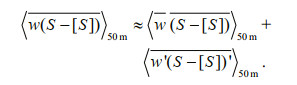
(3)where St is the salinity variation rate. Sv and Sw are the advective salt fluxes across the southern boundary and bottom boundary, respectively. Sydiff and Szdiff are the diffusive salt fluxes across the southern boundary and bottom boundary, respectively. SEP and SR are the evaporation minus precipitation and river runoff, respectively. [S] is time varying and volume-averaged salinity of the domain. This method was proposed by Lee et al. (2004) and has been widely used in heat and salt budget analysis (Zhang et al., 2018c; Lee et al., 2019; Soares et al., 2019). Details for the derivation of the box model for the salinity budget equation are given in Appendix A.
 (4)
(4)The eddy salt fluxes can be estimated by calculating the deviations from the time-averaged advective salt fluxes:
 (5)
(5) (6)
(6)For simplicity, 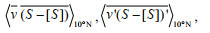
The above model product has been used in a series of studies: Li et al.(2016, 2018) and the present study. In Li et al. (2016), the model product has been validated with the Argo data and the SODA reanalysis dataset in terms of sea surface salinity anomalies in the tropical Indian Ocean. In Li et al. (2018), the observational and reanalysis data including the Argo data, the Research Moored Array for African-AsianAustralian monsoon analysis and prediction (RAMA), and the European Centre for Medium-Range Weather Forecasts (ECMWF) Ocean Reanalysis System 4 (ORAS4) have been used in the model validation for temperature, salinity, and zonal current anomalies along the equatorial Indian Ocean.
In the present study, the modeled currents and SSS are validated against the observational data. We choose January and July as the representative months for the winter and summer monsoons, respectively, to validate the model performance in terms of the sea surface circulation seasonality (Fig. 2) and the SSS (Fig. 3).

|
| Fig.2 Monthly-averaged surface horizontal currents in the BoB derived from drifter data in January (a), ROMS data in January (b), drifter data in July (c), and ROMS data in July (d) |

|
| Fig.3 Monthly averaged SSS in 2014 in the BoB derived from Argo data in January (a), ROMS data in January (b), Argo data in July (c), and ROMS data in July (d) |
Figure 2a-b display the monthly-averaged horizontal currents during the winter monsoon from drifter and ROMS data, respectively. It can be seen that ROMS reproduces the spatial distribution of the surface currents: a cyclonic circulation north of 15°N, the southward EICC southward of 18°N and a strong northward incoming flow at the southern boundary (about 10°N). However, the ROMS outputs underestimate the southward EICC and the circulation in the AS.
Figure 2c-d plot the monthly-averaged horizontal currents during the summer monsoon from the drifter and ROMS data, respectively. A similar general spatial distribution of the surface currents can also be seen: an anticyclonic circulation northward of 15°N, the southward EICC south of 15°N, a strong northward outflow at the southern boundary (around 85°E) and an approximately eastward flow east of 87°E. Similar to the winter monsoon comparison, the ROMS outputs also underestimate the EICC all along the western coast of the bay and the flow along the eastern coast, and overestimate the anticyclonic circulation in the northern bay area.
To further validate the model performance in terms of the climatological circulation simulation at the sea surface, the climatological model outputs (between 1982-2014) are compared with the drifter data (not shown). Even though there are differences in magnitude and along the west coast, the numerical results are consistent with the drifter data in terms of the spatial distribution patterns: in the northern BoB, the model reproduces the cyclonic (anticyclonic) gyre in summer (winter).
Many factors could contribute to the errors between the modeled and the drifter-derived circulations in this area. Firstly, the model is forced by 6-hourly wind field at the sea surface from the CFSv2 data in 2014, which could carry uncertainties for the oceanic circulation, especially in summer, when the local extreme weather conditions cannot be reproduced by the global model. Secondly, the drifter data used for the comparison are the climatological data, which are not a single-year oceanic circulation as presented in this study for the year 2014. Moreover, the number of the drifter records used in this set of observational data is small and unevenly distributed in the BoB, especially along the coastal region (Fig. 1 in Laurindo et al., 2017). Such insufficiency in the statistical sampling number could severely affect the reliability in the circulation in the southwest of the BoB, which could be the major reason for the inconsistent results in the comparison between the modeled and the drifter-derived circulations in the area.
Compared to Argo data, the ROMS model reproduces the SSS spatial distribution, albeit a slight overestimation of less than 0.6 over most of the region, except in the AS where a small underestimation of ~0.2 (absolute deviation value) is observed (Fig. 4). Compared with previous numerical simulations of SSS in the same area (Akhil et al., 2014; Wilson and Riser, 2016), the current results exhibit smaller errors. The good agreement between the ROMS and Argo data justifies the application of the model results in the present study.

|
| Fig.4 Annually averaged SSS in 2014 in the BoB derived from Argo (a) and ROMS data (b); SSS difference between the ROMS and Argo data (model data minus buoy data) (c); histogram of the SSS deviation of ROMS outputs from the Argo data (d) |
As shown in Fig. 3, salinity from both the model and Argo data shows a freshwater tongue extending from the east of the bay all the way to the west of the bay in January, but the freshwater tongue disappears in July. Instead, the salinity gradually decreases northeastward in July. Although the model results are in agreement with observation, there are discrepancies between the two data, especially north of 15°N. A possible explanation is that the ROMS model is forced with climatological river runoffs from CGDL, which is different from the river discharge in 2014.
To further validate the model performance in terms of the salinity simulation, we also make the comparison of the salinity vertical distribution in the domain with the BOA-Argo data (not shown), and the results show that the model reproduces the similar pattern as the observation.
3.2 Salinity variance balanceThe comparison of the time series for the terms on the two sides of Eq.1 shows good agreement (Fig. 5). The correlation coefficient between the salinitychanging-rate term (left side of the equation) and the sum of all influencing terms (right side of the equation) is 0.99, which means that the left and right sides of the equation are highly correlated. The root-mean-square error between the two sides of the equation is 0.09×10⁻², which is negligible as compared to the terms of Eq.1 in magnitude of 1×10⁻². Although St is slightly larger than the sum of all influencing terms from February to April, it is within the acceptable error range. The change in total salt volume (Stotal) shows a sharp decrease during the summer monsoon and increase during the winter monsoon. The change in salinity is not significant during the inter-monsoon periods (Fig. 5).

|
| Fig.5 Comparison between the two sides of Eq.1 (blue line: left side of the equation, red line: right side of the equation) and salinity variation (black line) in the upper 50 m of the BoB in 2014 The y-axis on the left side is for the blue and red lines, and the y-axis on the right side is for the black line. The correlation coefficient (Corr) between the salinity changing-rate term (left side of the equation) and the sum of all influencing terms (right side of the equation) is 0.99, and the root-meansquare error (RMSE) between the two sides of the equation is 0.09×10⁻². |
SEP, the evaporation minus precipitation term, is the dominant factor resulting in the sharp salinity decrease in the upper BoB (Fig. 6b), and it presents a significant positive correlation of 0.97 (not shown) with St (Fig. 6a). During the winter monsoon and early spring inter-monsoon (January to April), SEP is positive, which means that evaporation is larger than precipitation, thus causing an increase in salinity. From May to November (mainly including the summer monsoon and autumn inter-monsoon), SEP is negative, which suggests that precipitation is more than evaporation, hence resulting in the sharp decrease in salinity. SEP reaches its minimum value in July when the region experiences heavy rain. Overall, the trend of SEP resembles that of St, suggesting that it contributes significantly to the change of St (Fig. 6a).

|
| Fig.6 Monthly (a) and annual (b) averages of salinity budget terms St is the salinity variation rate (black line); Sv (magenta bars) and Sw (red bars) are the advective salt fluxes across the southern boundary and the bottom boundary, respectively. Sydiff (yellow bars) and Szdiff (orange bars) are the diffusive salt fluxes across the southern boundary and the bottom boundary, respectively. SEP (dark blue bars) and SR (light blue bars) are the evaporation-minus-precipitation and river runoff, respectively. |
SR, the river runoff, is the other significant factor making the decrease of the salinity in the BoB (Fig. 6b). It also has a similar trend to that of both St and SEP, but the freshwater injection is smaller than in SEP (Fig. 6a).
Therefore, the large net freshwater flux during the summer monsoon, especially the precipitation, is one of the main factors leading to the sharp salinity decrease in the upper BoB.
3.3.2 Effects of advectionSv, the meridional advective salt flux across the southern boundary, is the most important process that balances the excess precipitation and runoff over the full annual cycle (Fig. 6b). It is usually positive and becomes the most considerable term among all the influencing factors during the winter monsoon, reaching its peak in December and January and playing a leading role in increasing the salinity in the bay (Fig. 6a). During this period, the strong southward EICC transports a relatively salty water out of the bay. A northward flow carries salty water into the BoB through the middle area of the 10°N section between 81°E and 95°E, which is saltier than the water exported southward by the EICC. Moreover, the transport is stronger in the upper 30 m (Fig. 7a). In the eastern AS, a southward current exports the relatively fresh water out of the bay.
The magnitude of Sv decreases sharply during the spring inter-monsoon (Fig. 6a). During this period, the EICC shifts to a northward current with salty water injection (Fig. 7b). A negative advective salt flux appears between 81°E and 89°E because of the southward flow and positive salinity difference, while a positive salt flux comes up between 89°E and 92°E because the salinity difference turns to negative. The northward current transports fresher water into the AS, resulting in a net salinity decrease (Fig. 7b).

|
| Fig.7 Seasonally-averaged meridional velocity (v, shaded) effects on the salinity difference (S-[S], lines) at the southern boundary in the winter monsoon (a), the spring inter-monsoon (b), the summer monsoon (c), and the autumn inter-monsoon (d) in 2014 T hin full lines for positive values, thick full lines for zero values, and dashed lines for negative values. Negative and positive values denote the southward and northward velocity, respectively. |
Sv remains negative and presents a minimal magnitude in the early summer monsoon (June to July). It changes to positive in late summer monsoon, balancing the salinity freshening caused by the huge net freshwater injection (Fig. 6a). During this period, currents at the southern boundary are mostly southward except for the northward flow between 85°E and 96°E and below 20-m depth. The salinity difference mainly shows a positive pattern except for the AS, which in turn causes the negative salt flux basically located in the west of the southern boundary and the positive advective salt flux mostly located in the middle of the section below 20 m and the AS (Fig. 7c).
Sv is positive during the autumn inter-monsoon (Fig. 6a). During this period, the strong southward EICC transports the low-salinity water off the western BoB. A northward flow carries salty water through the middle area of the southern boundary between 83°E and 90°E. The southward currents along with the positive salinity difference induce a negative advective salt flux between 90°E and 94°E and the northward currents along with the negative salinity difference also induce a negative advective salt flux in the upper 40 m of the AS (Fig. 7d).
The annual mean of Sw, the advective salt flux across the bottom boundary, is smaller than Sv (Fig. 6b), while it is important especially during the monsoon seasons (December to February and June to July) to balance the salinity change induced by Sv (Fig. 6a). The vertical advective salt flux is sensitive to the Ekman pumping velocity (Ashin et al., 2019) at the depth of 50 m, that is,
 (7)
(7)and then is highly related to the wind stress curl. In Eq.7, f0 is the reference Coriolis parameter, ρ0 is the reference density of seawater, k is the vertical unit vector, and τ is the wind stress. To balance the positive (negative) wind stress curl, w|z=-50 cm must be upward (downward) according to Eq.7.
During the winter monsoon, Sw is significantly negative, making the upper bay fresher and counterbalancing the net northward advective salt flux at the southern boundary (Figs. 6a & 7a). The wind stress curl is mostly negative in the basin, except for the coastal region and the southern boundary of the study area (Fig. 8c). The negative wind stress, in turn, causes downwelling in the center of the bay, transporting the salty water out of the upper BoB at 50 m. The upwelling is concentrated along the eastern coast of the bay, carrying the fresher water upwards at 50 m (Fig. 8a). It should be noted that the salinity anomaly at the bottom boundary is derived from the time varying and volume-averaged salinity [S] of the domain. Due to this reason, even though the salinity generally increases with depth, an upwelling can transport water that is fresher than the control volume.

|
| Fig.8 Seasonally-averaged vertical velocity (w, shaded) effects on the salinity difference (S-[S], lines) at the bottom boundary (the upper row), and wind effects (vectors: wind stress; shading: wind stress curl) at the surface (the lower row) in winter monsoon (a, c) and summer monsoon (b, d) in 2014 Thin full lines for positive values, thick full lines for zero values, and dashed lines for negative values. Negative and positive w denote the downward and upward vertical velocity, respectively. |
During the summer monsoon, Sw is significantly positive, and counterbalance the negative advective salt flux due to the large freshwater injection, thus making the upper bay saltier (Fig. 6a). The wind stress curl is remarkably positive in the northern bay and along the western coast (Fig. 8d). It, in turn, causes upwelling in the northern and western bay, transporting the salty water into the upper BoB at 50 m (Fig. 8b).
3.3.3 Effects of turbulent diffusionsTurbulent diffusions also influence the salinity budget (Fig. 6b). Sydiff, the meridional diffusive salt flux across the southern boundary, becomes positive from June to December (Fig. 6a), balancing the sharp decrease of salinity during the summer monsoon and increasing it in the autumn inter-monsoon and early winter monsoon. Szdiff, the vertical diffusive salt flux across the bottom boundary, has a similar trend with Sw but with a smaller magnitude (Fig. 6a). It is also positive during the summer monsoon.
3.4 Eddy salt fluxesFor seasonal analysis, the advection can be decomposed into mean and eddy salt fluxes by applying Eqs.4 & 5. The spatial distribution of seasonally-averaged eddy salt fluxes at the interfaces reveals the detailed mesoscale structures of strong eddy signals (Figs. 9 & 10).

|
| Fig.9 Seasonally-averaged meridional eddy flux at the southern boundary during winter monsoon (a), spring inter-monsoon (b), summer monsoon (c), and autumn inter-monsoon (d) in 2014 |

|
| Fig.10 Seasonally-averaged vertical eddy flux at the bottom boundary during winter monsoon (a), spring inter-monsoon (b), summer monsoon (c), and autumn inter-monsoon (d) in 2014 The black line in (d) is the track of tropical cyclone HudHud on 7-13 October 2014 and the color dots are the position and intensity of the tropical cyclone (magenta: tropical depression; blue: tropical storm; green: typhoon). The best track data are from the Joint Typhoon Warning Center (https://www.metoc.navy.mil/jtwc/jtwc.html?north-indian-ocean). |
Sve, the eddy salt flux across the southern boundary, displays stronger eddy signals in the monsoon seasons than in the inter-monsoon seasons. Also, the positive eddy salt flux pattern exists near the western boundary throughout the year where the EICC located, and its magnitude is extremely large during the winter monsoon and the autumn inter-monsoon (Fig. 9). Sve is mostly positive during the winter monsoon and shows strong positive signatures on either side of the Andaman and Nicobar Islands (Figs. 1 & 9a). The absolute value of Sve decreases in the spring intermonsoon and eddy salt flux turns negative in the middle of the section below 30 m and beside the eastern boundary (Fig. 9b). Sve becomes strongly positive between 85°E and 90°E under the surface during the summer monsoon and shows abundant mesoscale signals east of 90°E (Fig. 9c). Sve decreases again in the autumn inter-monsoon except for the strong positive eddy salt flux near the western boundary. Other weaker eddy-flux signals are mainly concentrated in the upper 20 m and near the eastern boundary (Fig. 9d).
The spatial distribution of Swe (eddy salt flux across the bottom boundary) reveals abundant eddy-scale secondary salt flux circulation, with large magnitudes, except for the spring inter-monsoon (Fig. 10). During the winter monsoon, strong positive eddy salt flux can be found along the western coast and Swe is extremely negative around the Andaman and Nicobar Islands (Fig. 10a). A positive pattern is present between 80°E and 90°E in the southwestern BoB, and a weaker positive and negative value is observed in the middle of the bay during this period (Fig. 10a). During the spring inter-monsoon, the absolute value of Swe significantly decreases, while the eddy-scale signals are still obvious (Fig. 10b). During the summer monsoon, Swe makes a significantly negative contribution, especially along the western boundary and in the middle of the bay south of 15°N, while positive eddy salt flux can still be seen in the eastern bay, and around the Andaman and Nicobar Islands (Fig. 10c). During the autumn inter-monsoon, Swe plays a remarkable role in the western region of the BoB, with a negative eddy salt flux near the boundary and a positive flux in the middle of the bay (Fig. 10d). This strong eddy flux signal is caused by intensive upper-ocean mixing induced by the extremely severe tropical cyclone HudHud. From 7-13 October 2014, HudHud strengthened into a tropical storm near the Andaman and Nicobar Islands around 12°N, moved northwest, strengthened into a typhoon on 10 October, and made landfall on the east coast of India near 18°N (Fig. 10d), during which the maximum wind speed exceeded 50 m/s (Murty et al., 2020 and references therein).
4 DISCUSSIONIn the present study, we choose 2014 as a representative year to examine the seasonal salinity variations in the BoB. Given the strong seasonal variation in the BoB (controlled by the winter and summer monsoons), whose magnitude is much larger than the inter-annual variations, the analysis of the daily-sampled numerical outputs can shed more light on the understanding of the seasonal salinity variation.
Even though the 50-m depth of the BoB includes the upper mixed layer, it is useful to examine how the depth choice affects the salinity budget. We have conducted the calculation of the salinity budget for different bottom depths of the box (not shown). Sv is the main process that balances the surface freshwater input by the precipitation and river discharge in different depths in the upper BoB, although the magnitude of Sv decreases with increasing depth. Effects of Sw are different for different depths. It is the most important process that balances the excess precipitation and runoff over the full annual cycle in a shallower depth within the mixed layer, and gets smaller if the base of the control volume becomes deeper. Sydiff has a similar trend for all the different depths as tested, only the magnitude decreases as the depth increases. Szdiff is the term that has the greatest changes due to the choice of different depths, which causes the decrease (increase) of salinity in the shallower (deeper) depth.
The ROMS model is forced with the climatological data from the CGDL, with a lack of accurate river runoff forcing in the specific year. The arbitrary horizontal diffusivity set in the model required for the computational stability is another limitation, resulting in an overestimation of the horizontal diffusions.
At the sea surface, it is mainly the net freshwater flux that influences salinity transport, including SEP and SR. SEP increases salinity in the winter monsoon and spring inter-monsoon, and plays a leading role during the summer monsoon and autumn inter-monsoon, reducing the salinity by injecting a large amount of freshwater (Fig. 11c & d). SR decreases salinity in all seasons and its contribution is most significant during the summer monsoon and autumn inter-monsoon (Fig. 11).

|
| Fig.11 Seasonal salt transports during winter monsoon (a), spring inter-monsoon (b), summer monsoon (c), and autumn inter-monsoon (d) in the upper 50 m BoB in 2014 The transport (black numbers) calculation method is similar to the equations in Sections 2.4 & 2.5, except that the values are multiplied by the volume and the unit is Sv (1 Sv=106 m3/s). The percentages (red numbers) represent the proportion of the eddy salt transport to the absolute value of the total transport (i.e., the sum of the absolute value of eddy salt transport and seasonal mean transport). The red and blue arrows represent the salt transport into the control volume and salt transport out of the control volume, respectively. |
At the southern boundary, the seasonal mean meridional advective salt transport (Svm) generated by the background large-scale circulation, the meridional eddy salt flux (Sve) induced by the mesoscale signals and the meridional diffusive salt transport (Sydiff) caused by the sub-grid processes (e.g., small-scale eddies not resolved by the model) affect the salt transport. Svm dominates the salt transport during the winter monsoon, balancing the sharp salinity decrease induced by the large freshwater injection in the wet season (Fig. 11). Sve makes the salinity increase in all seasons, and the transport is strong (over 1 Sv) during the monsoon seasons (Fig. 11). In addition, the magnitude of Sve is sizeable (over 30%, Fig. 11) compared with the absolute value of the total meridional advective salt transport (i.e., the sum of the absolute value of Svm and Sve). Sydiff shows the positive diffusive salt transport throughout the year except for the spring inter-monsoon, and become significant in the summer monsoon and the autumn inter-monsoon (Fig. 11).
At the bottom boundary, the seasonal mean vertical advective salt transport (Swm) generated by the background large-scale circulation, the vertical eddy salt flux (Swe) induced by the mesoscale signals and the vertical diffusive salt transport (Szdiff) caused by the sub-grid processes affect the salt transport. Swm plays a significant role during monsoon seasons, making the salinity increase (decrease) during the summer (winter) monsoon (Fig. 11a & c). Swe makes the salinity increase in all seasons except for the summer monsoon. Though the total magnitude of Swe is smaller than Sve, it cannot be neglected (about 10%- 30%) compared with the absolute value of the total vertical advective salt transport (i.e., the sum of the absolute value of Swm and Swe), especially during the summer monsoon and the autumn inter-monsoon (Fig. 11). Szdiff shows the positive (negative) diffusive salt transport in the spring (autumn) inter-monsoon and summer (winter) monsoon, and the magnitude of Szdiff is comparable with Swe (Fig. 11).
The above results show that the horizontal eddy flux is larger than the vertical eddy flux (Fig. 11). One possible reason is the low vertical (~10 m in most regions of the upper 50 m) resolutions of the model outputs, which underestimates the influence of unresolved eddy fluxes. Another possibility is that the KPP scheme cannot describe all the sub-grid processes accurately, such as the mixed layer submesoscale motions, Langmuir circulation and the mixing induced by strong tropical cyclones. Similarly, the vertical diffusive salt flux could also be underestimated due to the lack of vertical resolution of the model.
5 CONCLUSIONIn this study, the factors influencing the salinity budget, including eddy salt fluxes, are analyzed in a fixed box model of the upper BoB in 2014, using daily averaged outputs from ROMS. The control volume is taken as the upper 50 m of the BoB, north of 10°N and the three open boundaries are the 10°N section, the sea surface and the 50-m level. The salinity budget indicates that the time series on the two sides of Eq.1 are balanced within the acceptable error range.
The salinity budget analysis demonstrates that the net freshwater flux is the dominant factor leading to the sharp salinity decrease during the summer monsoon. The advections, especially the meridional advective salt flux, are the main factors that cause the salinity to rise steadily after the summer monsoon, primarily affected by seasonal changes in circulations. The vertical advective salt flux plays an important role in balancing the salinity change induced by meridional advective salt flux during the monsoon seasons. In the winter monsoon, the downward advective salt flux at 50-m depth balances the northward high salinity flow into the bay at the southern boundary, while the opposite phenomenon exists in the summer monsoon. The downward (upward) vertical advective salt flux is caused by the negative (positive) wind stress curl during the winter (summer) monsoon. Turbulent diffusions can also influence the salinity budget. The meridional diffusive salt flux balances the sharp decrease of salinity during the summer monsoon and increases it in the autumn inter-monsoon and early winter monsoon. The vertical diffusive salt flux is also positive during the summer monsoon.
The eddy salt flux is decomposed to analyze its contribution. The spatial distributions of eddy salt fluxes show the distinctive mesoscale structures in all seasons, which magnitude is sizeable (over 30% for the meridional eddy salt flux and about 10%-30% for the vertical eddy salt flux). The eddy salt flux across the southern boundary displays stronger eddy signals during the monsoon seasons than during the inter-monsoon seasons, and is strongly positive near the west boundary where the EICC is located during the winter monsoon and autumn inter-monsoon. The eddy salt flux across the bottom boundary shows abundant eddy-scale signals, and is especially strong along the coast area and around the Andaman and Nicobar Islands. Strong eddy flux signals can be seen during the autumn inter-monsoon because of the tropical cyclonic HudHud causing intensive mixing in the upper ocean.
6 DATA AVAILABILITY STATEMENTThe datasets generated and/or analyzed for the current study are available from the corresponding author.
7 ACKNOWLEDGMENTThe BOA-Argo dataset used in this study is produced by the China Argo Real-time Data Center. These data were collected and made freely available by the International Argo Program and the national programs that contribute to it (http://www.argo.ucsd.edu, http://argo.jcommops.org). The Argo Program is part of the Global Ocean Observing System. The Drifter-Derived Climatology of Global Near-Surface Currents data are from ftp://ftp.aoml.noaa.gov/phod/pub/lumpkin/drifter_climatology. The best track data are from the Joint Typhoon Warning Center (https://www.metoc.navy.mil/jtwc/jtwc.html?north-indian-ocean).
Akhil V P, Durand F, Lengaigne M, Vialard J, Keerthi M G, Gopalakrishna V V, Deltel C, Papa F, de Boyer Montégut C. 2014. A modeling study of the processes of surface salinity seasonal cycle in the Bay of Bengal. Journal of Geophysical Research: Oceans, 119(6): 3 926-3 947.
DOI:10.1002/2013jc009632 |
Akhil V P, Lengaigne M, Vialard J, Durand F, Keerthi M G, Chaitanya A V S, Papa F, Gopalakrishna V V, de Boyer Montégut C. 2016. A modeling study of processes controlling the Bay of Bengal sea surface salinity interannual variability. Journal of Geophysical Research: Oceans, 121(12): 8 471-8 495.
DOI:10.1002/2016jc011662 |
Ashin K, Girishkumar M S, Suprit K, Thangaprakash V P. 2019. Observed upper ocean seasonal and intraseasonal variability in the Andaman Sea. Journal of Geophysical Research: Oceans, 124(10): 6 760-6 786.
DOI:10.1029/2019jc014938 |
Bouma T J, van Duren L A, Temmerman S, Claverie T, Blanco-Garcia A, Ysebaert T, Herman P M J. 2007. Spatial flow and sedimentation patterns within patches of epibenthic structures: combining field, flume and modelling experiments. Continental Shelf Research, 27(8): 1 020-1 045.
DOI:10.1016/j.csr.2005.12.019 |
Carton J A, Giese B S. 2008. A reanalysis of ocean climate using simple ocean data assimilation (SODA). Monthly Weather Review, 136(8): 2 999-3 017.
DOI:10.1175/2007MWR1978.1 |
Chen C S, Huang H S, Beardsley R C, Liu H D, Xu Q C, Cowles G. 2007. A finite volume numerical approach for coastal ocean circulation studies: comparisons with finite difference models. Journal of Geophysical Research, 112(C3): C03018.
DOI:10.1029/2006jc003485 |
Chen G X, Wang D X, Hou Y J. 2012. The features and interannual variability mechanism of mesoscale eddies in the Bay of Bengal. Continental Shelf Research, 47: 178-185.
DOI:10.1016/j.csr.2012.07.011 |
Dong C M, McWilliams J C, Liu Y, Chen D. 2014. Global heat and salt transports by eddy movement. Nature Communications, 5: 3 294.
DOI:10.1038/ncomms4294 |
Dong C M, McWilliams J C, Shchepetkin A F. 2007. Island wakes in deep water. Journal of Physical Oceanography, 37(4): 962-981.
DOI:10.1175/jpo3047.1 |
Gonaduwage L P, Chen G X, McPhaden M J, Priyadarshana T, Huang K, Wang D X. 2019. Meridional and zonal eddy-induced heat and salt transport in the Bay of Bengal and their seasonal modulation. Journal of Geophysical Research: Oceans, 124(11): 8 079-8 101.
DOI:10.1029/2019jc015124 |
Gopalan A K S, Krishna V V G, Ali M M, Sharma R. 2000. Detection of Bay of Bengal eddies from TOPEX and in situ observations. Journal of Marine Research, 58(5): 721-734.
DOI:10.1357/002224000321358873 |
Gulakaram V S, Vissa N K, Bhaskaran P K. 2020. Characteristics and vertical structure of oceanic mesoscale eddies in the Bay of Bengal. Dynamics of Atmospheres and Oceans, 89: 101131.
DOI:10.1016/j.dynatmoce.2020.101131 |
Han W Q, McCreary Jr J P. 2001. Modeling salinity distributions in the Indian Ocean. Journal of Geophysical Research: Oceans, 106(C1): 859-877.
DOI:10.1029/2000jc000316 |
Hormann V, Centurioni L R, Gordon A L. 2019. Freshwater export pathways from the Bay of Bengal. Deep Sea Research Part II: Topical Studies in Oceanography, 168: 104645.
DOI:10.1016/j.dsr2.2019.104645 |
Hu K L, Ding P X, Wang Z H, Yang S L. 2009. A 2D/3D hydrodynamic and sediment transport model for the Yangtze Estuary, China. Journal of Marine Systems, 77(1-2): 114-136.
DOI:10.1016/j.jmarsys.2008.11.014 |
Jacox M G, Hazen E L, Zaba K D, Rudnick D L, Edwards C A, Moore A M, Bograd S J. 2016. Impacts of the 2015-2016 El Niño on the California Current System: early assessment and comparison to past events. Geophysical Research Letters, 43(13): 7 072-7 080.
DOI:10.1002/2016gl069716 |
Jana S, Gangopadhyay A, Chakraborty A. 2015. Impact of seasonal river input on the Bay of Bengal simulation. Continental Shelf Research, 104: 45-62.
DOI:10.1016/j.csr.2015.05.001 |
Köhler J, Serra N, Bryan F O, Johnson B K, Stammer D. 2018. Mechanisms of mixed-layer salinity seasonal variability in the Indian Ocean. Journal of Geophysical Research: Oceans, 123(1): 466-496.
DOI:10.1002/2017jc013640 |
Large W G, McWilliams J C, Doney S C. 1994. Oceanic vertical mixing: a review and a model with a nonlocal boundary layer parameterization. Reviews of Geophysics, 32(4): 363-403.
DOI:10.1029/94RG01872 |
Laurindo L C, Mariano A J, Lumpkin R. 2017. An improved near-surface velocity climatology for the global ocean from drifter observations. Deep Sea Research Part I: Oceanographic Research Papers, 124: 73-92.
DOI:10.1016/j.dsr.2017.04.009 |
Lee T, Fournier S, Gordon A L, Sprintall J. 2019. Maritime Continent water cycle regulates low-latitude chokepoint of global ocean circulation. Nature Communications, 10(1): 2103.
DOI:10.1038/s41467-019-10109-z |
Lee T, Fukumori I, Tang B. 2004. Temperature advection: internal versus external processes. Journal of Physical Oceanography, 34(8): 1 936-1 944.
DOI:10.1175/1520-0485(2004)034<1936:Taivep>2.0.Co;2 |
Lekha J S, Buckley J M, Tandon A, Sengupta D. 2018. Subseasonal dispersal of freshwater in the northern Bay of Bengal in the 2013 Summer Monsoon Season. Journal of Geophysical Research: Oceans, 123(9): 6 330-6 348.
DOI:10.1029/2018jc014181 |
Li J D, Liang C J, Tang Y M, Dong C M, Chen D, Liu X H, Jin W F. 2016. A new dipole index of the salinity anomalies of the tropical Indian Ocean. Scientific Reports, 6: 24260.
DOI:10.1038/srep24260 |
Li J D, Liang C J, Tang Y M, Liu X H, Lian T, Shen Z Q, Li X J. 2018. Impacts of the IOD-associated temperature and salinity anomalies on the intermittent equatorial undercurrent anomalies. Climate Dynamics, 51(4): 1 391-1 409.
DOI:10.1007/s00382-017-3961-x |
Li Y L, Han W Q, Ravichandran M, Wang W Q, Shinoda T, Lee T. 2017. Bay of Bengal salinity stratification and Indian summer monsoon intraseasonal oscillation: 1. Intraseasonal variability and causes. Journal of Geophysical Research: Oceans, 122(5): 4 291-4 311.
DOI:10.1002/2017jc012691 |
Lin X Y, Qiu Y, Sun D Z. 2019. Thermohaline structures and heat/freshwater transports of mesoscale eddies in the Bay of Bengal Observed by Argo and satellite data. Remote Sensing, 11(24): 2989.
DOI:10.3390/rs11242989 |
Lu S L, Liu Z H, Li H, Li Z Q, Wu X F, Sun C H, Xu J P. 2020. User Manual of global ocean Argo gridded dataset (BOAArgo), 28, ftp://data.argo.org.cn/pub/ARGO/BOA_Argo/doc/BOA_Argo_readme_CN_2020.pdf. Accessed on 2020-7-23. (in Chinese)
|
Meijers A J, Bindoff N L, Roberts J L. 2007. On the total, mean, and eddy heat and freshwater transports in the Southern Hemisphere of a \({{\raise0.5ex\hbox{$\scriptstyle 1$} \kern-0.1em/\kern-0.15em \lower0.25ex\hbox{$\scriptstyle 8$}}. \circ } \times {{\raise0.5ex\hbox{$\scriptstyle 1$} \kern-0.1em/\kern-0.15em \lower0.25ex\hbox{$\scriptstyle 8$}}. \circ }\) global ocean model. Journal of Physical Oceanography, 37(2): 277-295.
DOI:10.1175/jpo3012.1 |
Murty P L N, Rao A D, Srinivas K S, Rao E P R, Bhaskaran P K. 2020. Effect of wave radiation stress in storm surge-induced inundation: a case study for the East Coast of India. Pure and Applied Geophysics, 177(6): 2 993-3 012.
DOI:10.1007/s00024-019-02379-x |
Narvekar J, Prasanna Kumar S. 2014. Mixed layer variability and chlorophyll a biomass in the Bay of Bengal. Biogeosciences, 11(14): 3 819-3 843.
DOI:10.5194/bg-11-3819-2014 |
Pant V, Girishkumar M S, Udaya Bhaskar T V S, Ravichandran M, Papa F, Thangaprakash V P. 2015. Observed interannual variability of near-surface salinity in the Bay of Bengal. Journal of Geophysical Research: Oceans, 120(5): 3315-3329.
DOI:10.1002/2014jc010340 |
Rao R R, Sivakumar R. 2003. Seasonal variability of sea surface salinity and salt budget of the mixed layer of the north Indian Ocean. Journal of Geophysical Research, 108(C1): 3009.
DOI:10.1029/2001jc000907 |
Saha S, Moorthi S, Pan H L, Wu X R, Wang J D, Nadiga S, Tripp P, Kistler R, Woollen J, Behringer D, Liu H X, Stokes D, Grumbine R, Gayno G, Wang J, Hou Y T, Chuang H Y, Juang H M H, Sela J, Iredell M, Treadon R, Kleist D, Van Delst P, Keyser D, Derber J, Ek M, Meng J, Wei H, Yang R Q, Lord S, van den Dool H, Kumar A, Wang W Q, Long C, Chelliah M, Xue Y, Huang B Y, Schemm J K, Ebisuzaki W, Lin R, Xie P P, Chen M Y, Zhou S T, Higgins W, Zou C Z, Liu Q H, Chen Y, Han Y, Cucurull L, Reynolds R W, Rutledge G, Goldberg M. 2010. The NCEP climate forecast system reanalysis. Bulletin of the American Meteorological Society, 91(8): 1 015-1 058.
DOI:10.1175/2010bams300L1 |
Saha S, Moorthi S, Wu X R, Wang J D, Nadiga S, Tripp P, Behringer D, Hou Y T, Chuang H Y, Iredell M, Ek M, Meng J, Yang R Q, Mendez M P, van den Dool H, Zhang Q, Wang W Q, Chen M, Becker E. 2014. The NCEP climate forecast system version 2. Journal of Climate, 27(6): 2 185-2 208.
DOI:10.1175/jcli-d-12-00823.1 |
Sandeep K K, Pant V, Girishkumar M S, Rao A D. 2018. Impact of riverine freshwater forcing on the sea surface salinity simulations in the Indian Ocean. Journal of Marine Systems, 185: 40-58.
DOI:10.1016/j.jmarsys.2018.05.002 |
Sanilkumar K V, Kuruvilla T V, Jogendranath D, Rao R R. 1997. Observations of the Western Boundary Current of the Bay of Bengal from a hydrographic survey during March 1993. Deep Sea Research Part I: Oceanographic Research Papers, 44(1): 135-145.
DOI:10.1016/S0967-0637(96)00036-2 |
Schott F A, McCreary Jr J P. 2001. The monsoon circulation of the Indian Ocean. Progress in Oceanography, 51(1): 1-123.
DOI:10.1016/S0079-6611(01)00083-0 |
Sengupta D, Bharath Raj G N, Shenoi S S C. 2006. Surface freshwater from Bay of Bengal runoff and Indonesian Throughflow in the tropical Indian Ocean. Geophysical Research Letters, 33(22): L22609.
DOI:10.1029/2006gl027573 |
Shee A, Sil S, Gangopadhyay A, Gawarkiewicz G, Ravichandran M. 2019. Seasonal evolution of oceanic upper layer processes in the Northern Bay of Bengal following a single Argo float. Geophysical Research Letters, 46(10): 5 369-5 377.
DOI:10.1029/2019gl082078 |
Sherin V R, Durand F, Papa F, Islam A S, Gopalakrishna V V, Khaki M, Suneel V. 2020. Recent salinity intrusion in the Bengal delta: observations and possible causes. Continental Shelf Research, 202: 104142.
DOI:10.1016/j.csr.2020.104142 |
Shetye S R, Gouveia A D, Shankar D, Shenoi S S C, Vinayachandran P N, Sundar D, Michael G S, Nampoothiri G. 1996. Hydrography and circulation in the western Bay of Bengal during the northeast monsoon. Journal of Geophysical Research: Oceans, 101(C6): 14 011-14 025.
DOI:10.1029/95jc03307 |
Soares S M, Richards K J, Bryan F O, Yoneyama K. 2019. On the seasonal cycle of the tropical South Indian Ocean. part Ⅰ: mixed layer heat and salt budgets. Journal of Climate, 32(6): 1 951-1 972.
DOI:10.1175/jcli-d-18-0036.1 |
Thompson B, Gnanaseelan C, Salvekar P S. 2006. Variability in the Indian Ocean circulation and salinity and its impact on SST anomalies during dipole events. Journal of Marine Research, 64(6): 853-880.
DOI:10.1357/002224006779698350 |
Trott C B, Subrahmanyam B, Murty V S N, Shriver J F. 2019a. Large-scale fresh and salt water exchanges in the Indian Ocean. Journal of Geophysical Research: Oceans, 124(8): 6 252-6 269.
DOI:10.1029/2019jc015361 |
Trott C B, Subrahmanyam B, Roman-Stork H L, Murty V S N, Gnanaseelan C. 2019b. Variability of intraseasonal oscillations and synoptic signals in sea surface salinity in the Bay of Bengal. Journal of Climate, 32(20): 6 703-6 728.
DOI:10.1175/jcli-d-19-0178.1 |
Vinayachandran P N, Shankar D, Vernekar S, Sandeep K K, Amol P, Neema C P, Chatterjee A. 2013. A summer monsoon pump to keep the Bay of Bengal salty. Geophysical Research Letters, 40(9): 1 777-1 782.
DOI:10.1002/grl.50274 |
Wilson E A, Riser S C. 2016. An assessment of the seasonal salinity budget for the upper Bay of Bengal. Journal of Physical Oceanography, 46(5): 1 361-1 376.
DOI:10.1175/jpo-d-15-0147.1 |
Xue P F, Chen C S, Ding P X, Beardsley R C, Lin H C, Ge J Z, Kong Y Z. 2009. Saltwater intrusion into the Changjiang River: a model-guided mechanism study. Journal of Geophysical Research, 114(C2): C02006.
DOI:10.1029/2008jc004831 |
Zhang C, Hou Y J, Li J. 2018a. Wave-current interaction during Typhoon Nuri (2008) and Hagupit (2008): an application of the coupled ocean-wave modeling system in the northern South China Sea. Journal of Oceanology and Limnology, 36(3): 663-675.
DOI:10.1007/s00343-018-6088-y |
Zhang Y L, Baptista A M. 2008. SELFE: a semi-implicit Eulerian-Lagrangian finite-element model for cross-scale ocean circulation. Ocean Modelling, 21(3-4): 71-96.
DOI:10.1016/j.ocemod.2007.11.005 |
Zhang Y L, Ye F, Stanev E V, Grashorn S. 2016. Seamless cross-scale modeling with SCHISM. Ocean Modelling, 102: 64-81.
DOI:10.1016/j.ocemod.2016.05.002 |
Zhang Y T, Xu H M, Qiao F L, Dong C M. 2018b. Seasonal variation of the global mixed layer depth: comparison between Argo data and FIO-ESM. Frontiers of Earth Science, 12(1): 24-36.
|
Zhang Y, Feng M, Du Y, Phillips H E, Bindoff N L, McPhaden M J. 2018c. Strengthened Indonesian throughflow drives decadal warming in the Southern Indian Ocean. Geophysical Research Letters, 45(12): 6 167-6 175.
DOI:10.1029/2018gl078265 |